- a
NorthFork Clip
- noaa.hub.arcgis.com
Updated Aug 24, 2022+ more versions Share
Share Facebook
 Twitter
 EmailClick to copy linkLink copiedCiteNOAA GeoPlatform (2022). NorthFork Clip [Dataset]. https://noaa.hub.arcgis.com/maps/731912b86f79415db4f402ea815211ae_1/aboutDataset updatedAug 24, 2022Dataset authored and provided byNOAA GeoPlatformArea coveredDescription
This is the flood extent map for the North Fork Black Creek for the specified stage using FESM.
- a
Defined Clip
- noaa.hub.arcgis.com
Updated Jan 5, 2021ShareFacebookTwitterEmailClick to copy linkLink copiedCiteNOAA GeoPlatform (2021). Defined Clip [Dataset]. https://noaa.hub.arcgis.com/datasets/noaa::bainbridge28ft-1?layer=1Dataset updatedJan 5, 2021Dataset authored and provided byNOAA GeoPlatformArea coveredDescriptionThis flood map was created using the HEC-RAS model by the US Army Corps of Engineers. The flood maps depict areas that are wet at specific stages. Water depth is not depicted.
- N
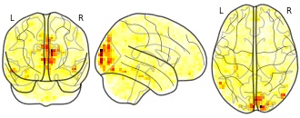
Movie clips: importance map LRP 5 Sadness
- neurovault.org
niftiUpdated Jan 9, 2018+ more versionsShareFacebookTwitterEmailClick to copy linkLink copiedCite(2018). Movie clips: importance map LRP 5 Sadness [Dataset]. http://identifiers.org/neurovault.image:58829niftiAvailable download formatsUnique identifierhttps://identifiers.org/neurovault.image:58829Dataset updatedJan 9, 2018LicenseCC0 1.0 Universal Public Domain Dedicationhttps://creativecommons.org/publicdomain/zero/1.0/
License information was derived automaticallyDescriptionFSL4.0
Collection description
Subject species
homo sapiens
Map type
Other
- a
Counties Clip
- gis-mhfd.hub.arcgis.com
- hub.arcgis.com
Updated Apr 17, 2020ShareFacebookTwitterEmailClick to copy linkLink copiedCiteMile High Flood District (2020). Counties Clip [Dataset]. https://gis-mhfd.hub.arcgis.com/datasets/mhfd::counties-clipDataset updatedApr 17, 2020Dataset authored and provided byMile High Flood DistrictArea coveredDescriptionThe Counties clipped layer was created using ArcGIS's Clip (Analysis) Tool to extract the DRCOG County Boundaries that overlay the MHFD District Boundary.
- N
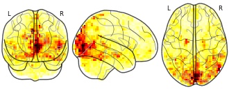
Movie clips: importance map OD 3 Happiness
- neurovault.org
niftiUpdated Jan 9, 2018+ more versionsShareFacebookTwitterEmailClick to copy linkLink copiedCite(2018). Movie clips: importance map OD 3 Happiness [Dataset]. http://identifiers.org/neurovault.image:58832niftiAvailable download formatsUnique identifierhttps://identifiers.org/neurovault.image:58832Dataset updatedJan 9, 2018LicenseCC0 1.0 Universal Public Domain Dedicationhttps://creativecommons.org/publicdomain/zero/1.0/
License information was derived automaticallyDescriptionFSL4.0
Collection description
Subject species
homo sapiens
Map type
Other
- m
Nanopore sequencing data (Chem-CLIP-MaP-seq)
- data.mendeley.com
Updated Jan 22, 2025ShareFacebookTwitterEmailClick to copy linkLink copiedCiteSherry Yang (2025). Nanopore sequencing data (Chem-CLIP-MaP-seq) [Dataset]. http://doi.org/10.17632/rszx769fn9.2Unique identifierhttps://doi.org/10.17632/rszx769fn9.2Dataset updatedJan 22, 2025AuthorsSherry YangLicenseAttribution 4.0 (CC BY 4.0)https://creativecommons.org/licenses/by/4.0/
License information was derived automaticallyDescriptionData for manuscript to be published about Chem-CLIP-MaP-seq
- N
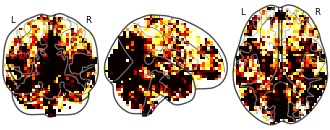
Movie clips: Reproducibility map OD p0.010 3 Happiness
- neurovault.org
niftiUpdated Jan 9, 2018+ more versionsShareFacebookTwitterEmailClick to copy linkLink copiedCite(2018). Movie clips: Reproducibility map OD p0.010 3 Happiness [Dataset]. http://identifiers.org/neurovault.image:58806niftiAvailable download formatsUnique identifierhttps://identifiers.org/neurovault.image:58806Dataset updatedJan 9, 2018LicenseCC0 1.0 Universal Public Domain Dedicationhttps://creativecommons.org/publicdomain/zero/1.0/
License information was derived automaticallyDescriptionFSL4.0
Collection description
Subject species
homo sapiens
Map type
Other
- a
GIS EXAM DCG-262-SEPT2023
- africageoportal.com
Updated Jul 21, 2025ShareFacebookTwitterEmailClick to copy linkLink copiedCiteAfrica GeoPortal (2025). GIS EXAM DCG-262-SEPT2023 [Dataset]. https://www.africageoportal.com/datasets/africageoportal::gis-exam-dcg-262-sept2023Dataset updatedJul 21, 2025Dataset authored and provided byAfrica GeoPortalDescriptionNDVI Analysis for Kiambu county. The NDVI was computed using Landsat 8 bands: NDVI=(Band 5(Nir)-Band 4(red))/(Band 5+Band4). The NDVI image was classified into four vegetation health classes. Each class was assigned a specific color using the Qgis symbology tools. The output was a ndvi Kiambu map.Land use Land cover Mapping. Combine all the satellite bands using the band set in the SCP.Landsat image bands were stacked using the Build Virtual Raster tool in QGIS.This formed a multispectral image for further analysis. Clip the image to area of extent. The study area was clipped the map canvas extent. Supervised Classification for LULC Map was performed using the Semi-Automatic Classification Plugin (SCP):Training samples were created for land cover classes: water, vegetation, built-up, bare land.Classification method used: Maximum LikelihoodA classified LULC map was produced, representing each pixel with its respective class.Output: clipped_stack.tif (study area image)
- d
DPD council districts shore clip - Absolute % Change
- catalog.data.gov
- data.seattle.gov
- +2more
Updated Apr 19, 2025+ more versionsShareFacebookTwitterEmailClick to copy linkLink copiedCiteCity of Seattle ArcGIS Online (2025). DPD council districts shore clip - Absolute % Change [Dataset]. https://catalog.data.gov/dataset/dpd-council-districts-shore-clip-absolute-changeDataset updatedApr 19, 2025Dataset provided byCity of Seattle ArcGIS OnlineDescriptionThis data layer references data from a high-resolution tree canopy change-detection layer for Seattle, Washington. Tree canopy change was mapped by using remotely sensed data from two time periods (2016 and 2021). Tree canopy was assigned to three classes: 1) no change, 2) gain, and 3) loss. No change represents tree canopy that remained the same from one time period to the next. Gain represents tree canopy that increased or was newly added, from one time period to the next. Loss represents the tree canopy that was removed from one time period to the next. Mapping was carried out using an approach that integrated automated feature extraction with manual edits. Care was taken to ensure that changes to the tree canopy were due to actual change in the land cover as opposed to differences in the remotely sensed data stemming from lighting conditions or image parallax. Direct comparison was possible because land-cover maps from both time periods were created using object-based image analysis (OBIA) and included similar source datasets (LiDAR-derived surface models, multispectral imagery, and thematic GIS inputs). OBIA systems work by grouping pixels into meaningful objects based on their spectral and spatial properties, while taking into account boundaries imposed by existing vector datasets. Within the OBIA environment a rule-based expert system was designed to effectively mimic the process of manual image analysis by incorporating the elements of image interpretation (color/tone, texture, pattern, location, size, and shape) into the classification process. A series of morphological procedures were employed to ensure that the end product is both accurate and cartographically pleasing. No accuracy assessment was conducted, but the dataset was subjected to manual review and correction.University of Vermont Spatial Analysis LaboratoryThis dataset consists of City of Seattle Council District areas as they existed in the first comparison year (2016) which cover the following tree canopy categories:Existing tree canopy percentPossible tree canopy - vegetation percentRelative percent changeAbsolute percent changeFor more information, please see the 2021 Tree Canopy Assessment.
- a
SRTM15 Gulf of Mexico clip (GCOOS)
- gcoos-tamu.opendata.arcgis.com
- gisdata.gcoos.org
- +1more
Updated Oct 1, 2019+ more versionsShareFacebookTwitterEmailClick to copy linkLink copiedCiteriles2@tamu.edu_tamu (2019). SRTM15 Gulf of Mexico clip (GCOOS) [Dataset]. https://gcoos-tamu.opendata.arcgis.com/content/7b2c266d4d1649a7967d20c1a4d9aaf3Dataset updatedOct 1, 2019Dataset authored and provided byriles2@tamu.edu_tamuLicenseMIT Licensehttps://opensource.org/licenses/MIT
License information was derived automaticallyArea coveredDescriptionThis dataset is the NOAA NCEI SRTM15+ v2.0 (29 March 2019) clipped to the area containing and immediately surrounding the Gulf of Mexico.To provide an improved mapping of the seafloor fabric globally, NOAA NCEI have used available sounding data along with an improved global marine gravity model to develop at grid at 15 arcsecond resolution (~500 m). Land elevations are based on the best available data from SRTM, ASTER digital elevation models while the ice topography of Greenland and Antarctica is based on CryoSat-2 and IceSat. Ocean bathymetry is based on bathymetric predictions from the latest global gravity model from CryoSat-2 and Jason-1 along with 494 million carefully edited depth soundings at 15 arcsecond resolution.NOAA NCEI have used the bathymetry grid along with the improved gravity to construct a global map of abyssal hill amplitude and orientations and compare the orientations with predictions from seafloor age gradient analysis. Areas of disagreement reveal propagating rifts, microplates, and tectonic reorganizations. This SRTM15_PLUS provides the foundational bathymetry layer for Google Earth and is freely available at NOAA NCEI ftp site (topex.ucsd.edu).
Rough Skate Footage
- kaggle.com
Updated Sep 5, 2025ShareFacebookTwitterEmailClick to copy linkLink copiedCiteAyush Rawat (2025). Rough Skate Footage [Dataset]. https://www.kaggle.com/icebearisin/raw-skates/activityCroissantCroissant is a format for machine-learning datasets. Learn more about this at mlcommons.org/croissant.Dataset updatedSep 5, 2025Dataset provided byKaggleAuthorsAyush RawatLicensehttp://www.gnu.org/licenses/old-licenses/gpl-2.0.en.htmlhttp://www.gnu.org/licenses/old-licenses/gpl-2.0.en.html
DescriptionContext
I had recently shifted to a new city, which completely lacks any skateboarding scene. So, I thought I'll finally realize my long-standing idea for (creating a bot for SkaterXL)[https://github.com/Marceline/SkateBrot]. This dataset got created from my initial tries/thoughts for the same. I quickly realized that labelling data is something that's crucial as well as time consuming. So, I made a habit of doing a little bit of it everyday, even though I knew that my methods might render most of it useless for actual consumption. But hey, you live and learn, and skate!
Content
So, there are two types of data here, real footage of skaters almost all of it from the same park(Berrics). And artificial Skate footage from SkaterXL. The real footage is made up of short(<10s) clips, consisting of exactly one trick. With the filename being that trick's name. Further, tricks with lots of representation have gotten their own subdirectories. This data is scarce, and is provided with the intention of being used for testing with respect to the real world. Artificial footage is meant to be trained on, and it contains three phases. The earliest is freeform footage from one of my friends playing SkaterXL. Then comes footage where clips show attempts at a particular line, i.e. they start from the same point in the map. Finally, come the part where each clip is paired with a csv file containing (grabbed) inputs for that clip.
Acknowledgements
The real footage comes from the Battle at the Berrics that I'd downloaded due to my ISPs being flakey. The SkaterXL footage is made possible by Tanyut Huidrom.
Inspiration
Note that all of the SkaterXL clips are technically self sufficient for training. The instantaneous input is represented by the in-game controller overlay(X) in the bottom-left, and tricks(y) are shown on top-left. But there are three problems. First is, that both overlays are translucent, and depend heavily on the map being played (which in themselves are colorfully diverse). Secondly, the controller-overlay has many different variants (only two in this dataset though). Finally, the in-game trick overlay is often not the label, as it can (very rarely) misidentify, is on-screen for a duration, and contains a history as well. The following are my task ideas, some of which I'm always trying to implement: 1. Given SkaterXL footage, and starting on the same map at the same location. Extract the controls that would generate it. 2. Do 1., but also validate by replaying the controls in the game for real. Note that SkaterXL only supports Windows (though, it's written in Unity)**If you have any idea on how I can do this playing-the-game on cloud, please do tell.** 3. Use the model thus trained to watch in-game skaters, and then predict the controls that will generate a different set of tricks, but go through approximately the same region on the game map. 4. Modify the model trained using above stuff to classify tricks in the actual footage. (Modify the above model, because labelling actual footage is hard, while SkaterXL footage has reasonably decent auto-labelling due to the Game).
Additional file 4 of Principles of RNA processing from analysis of enhanced...
- springernature.figshare.com
xlsxUpdated May 31, 2023ShareFacebookTwitterEmailClick to copy linkLink copiedCiteEric L. Van Nostrand; Gabriel A. Pratt; Brian A. Yee; Emily C. Wheeler; Steven M. Blue; Jasmine Mueller; Samuel S. Park; Keri E. Garcia; Chelsea Gelboin-Burkhart; Thai B. Nguyen; Ines Rabano; Rebecca Stanton; Balaji Sundararaman; Ruth Wang; Xiang-Dong Fu; Brenton R. Graveley; Gene W. Yeo (2023). Additional file 4 of Principles of RNA processing from analysis of enhanced CLIP maps for 150 RNA binding proteins [Dataset]. http://doi.org/10.6084/m9.figshare.12096759.v1xlsxAvailable download formatsUnique identifierhttps://doi.org/10.6084/m9.figshare.12096759.v1Dataset updatedMay 31, 2023AuthorsEric L. Van Nostrand; Gabriel A. Pratt; Brian A. Yee; Emily C. Wheeler; Steven M. Blue; Jasmine Mueller; Samuel S. Park; Keri E. Garcia; Chelsea Gelboin-Burkhart; Thai B. Nguyen; Ines Rabano; Rebecca Stanton; Balaji Sundararaman; Ruth Wang; Xiang-Dong Fu; Brenton R. Graveley; Gene W. YeoLicenseAttribution 4.0 (CC BY 4.0)https://creativecommons.org/licenses/by/4.0/
License information was derived automaticallyDescriptionAdditional file 4: Table S3. List of multi-copy element annotations used in family-aware mapping.
Geothermal Resource Potential by Field
- data.cnra.ca.gov
- data.ca.gov
- +5more
Updated Oct 3, 2024ShareFacebookTwitterEmailClick to copy linkLink copiedCiteCalifornia Energy Commission (2024). Geothermal Resource Potential by Field [Dataset]. https://data.cnra.ca.gov/dataset/geothermal-resource-potential-by-fieldxlsx, html, csv, zip, arcgis geoservices rest api, gpkg, geojson, kml, txt, gdbAvailable download formatsDataset updatedOct 3, 2024LicenseAttribution 4.0 (CC BY 4.0)https://creativecommons.org/licenses/by/4.0/
License information was derived automaticallyDescriptionThis data layer contains geothermal resource areas and their technical potential used in long-term electric system modeling for Integrated Resource Planning and SB 100. Geothermal resource areas are delineated by Known Geothermal Resource Areas (KGRAs) (Geothermal Map of California, 2002), other geothermal fields (CalGEM Field Admin Boundaries, 2020), and Bureau of Land Management (BLM) Geothermal Leasing Areas (California BLM State Office GIS Department, 2010). The fields that are considered in our assessment have enough information known about the geothermal reservoir that an electric generation potential was estimated by USGS (Williams et al. 2008) or estimated by a BLM Environmental Impact Statement (El Centro Field Office, 2007). For the USGS identified geothermal systems, any point that lies within 2 km of a field is summed to represent the total mean electrical generation potential from the entire field.
Geothermal field boundaries are constructed for identified geothermal systems that lie outside of an established geothermal field. A circular footprint is assumed with a radius determined by the area needed to support the mean resource potential estimate, assuming a 10 MW/km2 power density.
Several geothermal fields have power plants that are currently generating electricity from the geothermal source. The total production for each geothermal field is estimated by the CA Energy Commission’s Quarterly Fuel and Energy Report that tracks all power plants greater than 1 MW. The nameplate capacity of all generators in operation as of 2021 were used to inform how much of the geothermal fields are currently in use. This source yields inconsistent results for the power plants in the Geysers. Instead, an estimate from the net energy generation from those power plants is used. Using these estimates, the net undeveloped geothermal resource potential can be calculated.
Finally, we apply the protected area layer for geothermal to screen out those geothermal fields that lie entirely within a protected area. The protected area layer is compiled from public and private lands that have special designations prohibiting or not aligning with energy development.
This layer is featured in the CEC 2023 Land-Use Screens for Electric System Planning data viewer.
For more information about this layer and its use in electric system planning, please refer to the Land Use Screens Staff Report in the CEC Energy Planning Library.
Change Log:
Version 1.1 (January 18, 2024)
- ProtectedArea_Exclusion field was updated to correct for the changes to the Protected Area Layer. A Development Focus Area on Bureau of Land Management (BLM) land that overlays the Coso Hot Springs allows its resource potential to be considered in the statewide estimate.
Data Dictionary:
Total_MWe_Mean: The estimated resource potential from each geothermal field. All geothermal fields, except for Truckhaven, was given an estimate by Williams et al. 2008. If more than one point resource intersects (within 2km of) the field, the sum of the individual geothermal systems was used to estimate the magnitude of the resource coming from the entire geothermal field. Estimates are given in MW.
Total_QFER_NameplateCapacity: The total nameplate capacities of all generators in operation as of 2021 that intersects (within 2 km of) a geothermal field. The resource potential already in use for the Geysers is determined by Lovekin et al. 2004. Estimates are given in MW.
ProtectedArea_Exclusion: Binary value representing whether a field is excluded by the land-use screen or not. Fields that are excluded have a value of 1; those that aren’t have a value of 0.
NetUndevelopedRP: The net undeveloped resource potential for each geothermal field. This field is determined by subtracting the total resource potential in use (Total_QFER_NameplateCapacity) from the total estimated resource potential (Total_MWe_Mean). Estimates are given in MW.
Acres_GeothermalField: This is the geodesic acreage of each geothermal field. Values are reported in International Acres using a NAD 1983 California (Teale) Albers (Meters) projection.
References:
- Geothermal Map of California, S-11. California Department of Conservation, 2002. https://www.conservation.ca.gov/calgem/geothermal/maps/Pages/index.aspx
- CalGEM Field Admin Boundaries,
2020. https://gis.conservation.ca.gov/server/rest/services/CalGEM/Admin_Bounds/MapServer
- California BLM State Office GIS
Department, California BLM Verified and Potential Geothermal
Leases in California, 2010. https://databasin.org/datasets/5ec77a1438ab4402bf09ef9bfd7f04d9/
- Williams, Colin F., Reed, Marshall J., Mariner, Robert H., DeAngelo, Jacob, Galanis, S. Peter, Jr. 2008. "Assessment of moderate- and high-temperature geothermal resources of the United States: U.S. Geological Survey Fact Sheet 2008-3082." 4 p. https://certmapper.cr.usgs.gov/server/rest/services/geothermal/westus_favoribility_systems/MapServer/0
- El Centro Field Office, Bureau of Land Management (2007). Final Environmental Impact Statement for the Truckhaven Geothermal Leasing Area (Publication Index Number: BLM/CA/ES-2007-017+3200). United States Department of the Interior Bureau of Land Management.
- Lovekin, James W., Subir K. Sanyal, Christopher W. Klein. 2004. “New Geothermal Site Identification and Qualification.” Richmond, California:
- W
CalTrans Airport Runways
- wifire-data.sdsc.edu
- gis-calema.opendata.arcgis.com
csv, esri rest +4Updated May 17, 2019+ more versionsShareFacebookTwitterEmailClick to copy linkLink copiedCiteCA Governor's Office of Emergency Services (2019). CalTrans Airport Runways [Dataset]. https://wifire-data.sdsc.edu/dataset/caltrans-airport-runwayskml, esri rest, geojson, html, zip, csvAvailable download formatsDataset updatedMay 17, 2019Dataset provided byCA Governor's Office of Emergency ServicesLicenseCC0 1.0 Universal Public Domain Dedicationhttps://creativecommons.org/publicdomain/zero/1.0/
License information was derived automaticallyDescriptionThis feature layer is a line feature class representing the airport runways in California for which the Caltrans HQ Aeronautics maintains information. For planning purpose only
The maps and data are made available to the public solely for informational purposes. Information provided in the Caltrans GIS Data Library is accurate to the best of our knowledge and is subject to change on a regular basis, without notice. While the GIS Data Management Branch makes every effort to provide useful and accurate information, we do not warrant the information to be authoritative, complete, factual, or timely. Information is provided on an "as is" and an "as available" basis. The Department of Transportation is not liable to any party for any cost or damages, including any direct, indirect, special, incidental, or consequential damages, arising out of or in connection with the access or use of, or the inability to access or use, the Site or any of the Materials or Services described herein.
- N
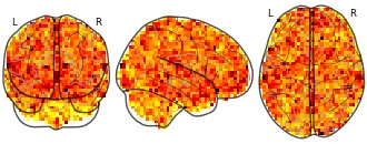
Movie clips: importance map W 2 Fear
- neurovault.org
niftiUpdated Jan 9, 2018+ more versionsShareFacebookTwitterEmailClick to copy linkLink copiedCite(2018). Movie clips: importance map W 2 Fear [Dataset]. http://identifiers.org/neurovault.image:58841niftiAvailable download formatsUnique identifierhttps://identifiers.org/neurovault.image:58841Dataset updatedJan 9, 2018LicenseCC0 1.0 Universal Public Domain Dedicationhttps://creativecommons.org/publicdomain/zero/1.0/
License information was derived automaticallyDescriptionFSL4.0
Collection description
Subject species
homo sapiens
Map type
Other
- W
Utilities Fire Threat Areas
- wifire-data.sdsc.edu
- hub.arcgis.com
- +3more
esri rest, htmlUpdated Sep 3, 2019+ more versionsShareFacebookTwitterEmailClick to copy linkLink copiedCiteCA Governor's Office of Emergency Services (2019). Utilities Fire Threat Areas [Dataset]. https://wifire-data.sdsc.edu/am/dataset/utilities-fire-threat-areashtml, esri restAvailable download formatsDataset updatedSep 3, 2019Dataset provided byCA Governor's Office of Emergency ServicesLicenseCC0 1.0 Universal Public Domain Dedicationhttps://creativecommons.org/publicdomain/zero/1.0/
License information was derived automaticallyDescriptionIn 2012, the CPUC ordered the development of a statewide map that is designed specifically for the purpose of identifying areas where there is an increased risk for utility associated wildfires. The development of the CPUC -sponsored fire-threat map, herein "CPUC Fire-Threat Map," started in R.08-11-005 and continued in R.15-05-006.
A multistep process was used to develop the statewide CPUC Fire-Threat Map. The first step was to develop Fire Map 1 (FM 1), an agnostic map which depicts areas of California where there is an elevated hazard for the ignition and rapid spread of powerline fires due to strong winds, abundant dry vegetation, and other environmental conditions. These are the environmental conditions associated with the catastrophic powerline fires that burned 334 square miles of Southern California in October 2007. FM 1 was developed by CAL FIRE and adopted by the CPUC in Decision 16-05-036.
FM 1 served as the foundation for the development of the final CPUC Fire-Threat Map. The CPUC Fire-Threat Map delineates, in part, the boundaries of a new High Fire-Threat District (HFTD) where utility infrastructure and operations will be subject to stricter fire‑safety regulations. Importantly, the CPUC Fire-Threat Map (1) incorporates the fire hazards associated with historical powerline wildfires besides the October 2007 fires in Southern California (e.g., the Butte Fire that burned 71,000 acres in Amador and Calaveras Counties in September 2015), and (2) ranks fire-threat areas based on the risks that utility-associated wildfires pose to people and property.
Primary responsibility for the development of the CPUC Fire-Threat Map was delegated to a group of utility mapping experts known as the Peer Development Panel (PDP), with oversight from a team of independent experts known as the Independent Review Team (IRT). The members of the IRT were selected by CAL FIRE and CAL FIRE served as the Chair of the IRT. The development of CPUC Fire-Threat Map includes input from many stakeholders, including investor-owned and publicly owned electric utilities, communications infrastructure providers, public interest groups, and local public safety agencies.
The PDP served a draft statewide CPUC Fire-Threat Map on July 31, 2017, which was subsequently reviewed by the IRT. On October 2 and October 5, 2017, the PDP filed an Initial CPUC Fire-Threat Map that reflected the results of the IRT's review through September 25, 2017. The final IRT-approved CPUC Fire-Threat Map was filed on November 17, 2017. On November 21, 2017, SED filed on behalf of the IRT a summary report detailing the production of the CPUC Fire-Threat Map(referenced at the time as Fire Map 2). Interested parties were provided opportunity to submit alternate maps, written comments on the IRT-approved map and alternate maps (if any), and motions for Evidentiary Hearings. No motions for Evidentiary Hearings or alternate map proposals were received. As such, on January 19, 2018 the CPUC adopted, via Safety and Enforcement Division's (SED) disposition of a Tier 1 Advice Letter, the final CPUC Fire-Threat Map.
Additional information can be found here.
- a
Inner Clip
- noaa.hub.arcgis.com
Updated Dec 6, 2022ShareFacebookTwitterEmailClick to copy linkLink copiedCiteNOAA GeoPlatform (2022). Inner Clip [Dataset]. https://noaa.hub.arcgis.com/datasets/47367874a38349cbac566b844fc2f2e4Dataset updatedDec 6, 2022Dataset authored and provided byNOAA GeoPlatformArea coveredDescriptionFESM Map for the St Marys River at the Specified stage
- f
Additional file 1 of Principles of RNA processing from analysis of enhanced...
- springernature.figshare.com
xlsxUpdated Jun 1, 2023ShareFacebookTwitterEmailClick to copy linkLink copiedCiteEric L. Van Nostrand; Gabriel A. Pratt; Brian A. Yee; Emily C. Wheeler; Steven M. Blue; Jasmine Mueller; Samuel S. Park; Keri E. Garcia; Chelsea Gelboin-Burkhart; Thai B. Nguyen; Ines Rabano; Rebecca Stanton; Balaji Sundararaman; Ruth Wang; Xiang-Dong Fu; Brenton R. Graveley; Gene W. Yeo (2023). Additional file 1 of Principles of RNA processing from analysis of enhanced CLIP maps for 150 RNA binding proteins [Dataset]. http://doi.org/10.6084/m9.figshare.12096735.v1xlsxAvailable download formatsUnique identifierhttps://doi.org/10.6084/m9.figshare.12096735.v1Dataset updatedJun 1, 2023Dataset provided byfigshareAuthorsEric L. Van Nostrand; Gabriel A. Pratt; Brian A. Yee; Emily C. Wheeler; Steven M. Blue; Jasmine Mueller; Samuel S. Park; Keri E. Garcia; Chelsea Gelboin-Burkhart; Thai B. Nguyen; Ines Rabano; Rebecca Stanton; Balaji Sundararaman; Ruth Wang; Xiang-Dong Fu; Brenton R. Graveley; Gene W. YeoLicenseAttribution 4.0 (CC BY 4.0)https://creativecommons.org/licenses/by/4.0/
License information was derived automaticallyDescriptionAdditional file 1: Table S1. Accession identifiers for eCLIP datasets used in the manuscript.
- f
Additional file 5 of Principles of RNA processing from analysis of enhanced...
- springernature.figshare.com
xlsxUpdated Jun 1, 2023ShareFacebookTwitterEmailClick to copy linkLink copiedCiteEric L. Van Nostrand; Gabriel A. Pratt; Brian A. Yee; Emily C. Wheeler; Steven M. Blue; Jasmine Mueller; Samuel S. Park; Keri E. Garcia; Chelsea Gelboin-Burkhart; Thai B. Nguyen; Ines Rabano; Rebecca Stanton; Balaji Sundararaman; Ruth Wang; Xiang-Dong Fu; Brenton R. Graveley; Gene W. Yeo (2023). Additional file 5 of Principles of RNA processing from analysis of enhanced CLIP maps for 150 RNA binding proteins [Dataset]. http://doi.org/10.6084/m9.figshare.12096765.v1xlsxAvailable download formatsUnique identifierhttps://doi.org/10.6084/m9.figshare.12096765.v1Dataset updatedJun 1, 2023Dataset provided byfigshareAuthorsEric L. Van Nostrand; Gabriel A. Pratt; Brian A. Yee; Emily C. Wheeler; Steven M. Blue; Jasmine Mueller; Samuel S. Park; Keri E. Garcia; Chelsea Gelboin-Burkhart; Thai B. Nguyen; Ines Rabano; Rebecca Stanton; Balaji Sundararaman; Ruth Wang; Xiang-Dong Fu; Brenton R. Graveley; Gene W. YeoLicenseAttribution 4.0 (CC BY 4.0)https://creativecommons.org/licenses/by/4.0/
License information was derived automaticallyDescriptionAdditional file 5: Table S4. Quantitation of multi-copy RNA family enrichment for 223 eCLIP datasets.
Wetlands (Hosted Tile Layer)
- data.ca.gov
- data.cnra.ca.gov
- +5more
Updated Mar 22, 2024ShareFacebookTwitterEmailClick to copy linkLink copiedCiteCalifornia Energy Commission (2024). Wetlands (Hosted Tile Layer) [Dataset]. https://data.ca.gov/dataset/wetlands-hosted-tile-layerarcgis geoservices rest api, htmlAvailable download formatsDataset updatedMar 22, 2024LicenseAttribution 4.0 (CC BY 4.0)https://creativecommons.org/licenses/by/4.0/
License information was derived automaticallyDescriptionThis dataset is available for download from: Wetlands (File Geodatabase).
Wetlands in California are protected by several federal and state laws, regulations, and policies. This layer was extracted from the broader land cover raster from the CA Nature project which was recently enhanced to include a more comprehensive definition of wetland. This wetlands dataset is used as an exclusion as part of the biological planning priorities in the CEC 2023 Land-Use Screens.
This layer is featured in the CEC 2023 Land-Use Screens for Electric System Planning data viewer.
For more information about this layer and its use in electric system planning, please refer to the Land Use Screens Staff Report in the CEC Energy Planning Library.
Change Log
Version 1.1 (January 26, 2023)
- Full resolution of wetlands replaced a coarser resolution version that was previously shared. Also, file type changed from polygon to raster (feature service to tile layer service).
FacebookTwitterThis is the flood extent map for the North Fork Black Creek for the specified stage using FESM.