Panel data, also known as longitudinal data, consist of a collection of time series. Each time series, which could itself be multivariate, comprises a sequence of measurements taken on a distinct unit. Mechanistic modeling involves writing down scientifically motivated equations describing the collection of dynamic systems giving rise to the observations on each unit. A defining characteristic of panel systems is that the dynamic interaction between units should be negligible. Panel models therefore consist of a collection of independent stochastic processes, generally linked through shared parameters while also having unit-specific parameters. To give the scientist flexibility in model specification, we are motivated to develop a framework for inference on panel data permitting the consideration of arbitrary nonlinear, partially observed panel models. We build on iterated filtering techniques that provide likelihood-based inference on nonlinear partially observed Markov process models for time series data. Our methodology depends on the latent Markov process only through simulation; this plug-and-play property ensures applicability to a large class of models. We demonstrate our methodology on a toy example and two epidemiological case studies. We address inferential and computational issues arising due to the combination of model complexity and dataset size. Supplementary materials for this article are available online.

This study is a longitudinal national data series for 167 nations. The present dataset represents an expansion both of temporal coverage and of substantive variable categories from the earlier CROSS POLITY TIME SERIES (ICPSR 5002) by the Center for Comparative Political Research, State University of New York (Binghamton). General areas included among the variables now available are demographic, social, political, and economic topics. Cases in the data collection represent nation-year observations. (Source: downloaded from ICPSR 7/13/10)

Please Note: This dataset is part of the historical CISER Data Archive Collection and is also available at ICPSR at https://doi.org/10.3886/ICPSR07412.v1. We highly recommend using the ICPSR version as they have made this dataset available in multiple data formats.

The Quarterly Workforce Indicators (QWI) are a set of economic indicators including employment, job creation, earnings, and other measures of employment flows. The QWI are reported using detailed firm characteristics (geography, industry, age, size) and worker demographics information (sex, age, education, race, ethnicity). For more information see http://lehd.ces.census.gov/data/#qwi

The Cross-National Time-Series (CNTS) Data Archive is a longitudinal dataset offering over 200 years of annual country-level data spanning from 1815 to 2024. Covering more than 200 nations, the dataset includes 196 variables across demographic, political, legislative, economic, social, and conflict-related domains. Researchers can analyze diverse topics, including socio-economic indicators, political stability, legislative effectiveness, international status rankings, urbanization, communication technologies, trade, military activity, education enrollment, and industrial production.

Abstract

The Russia Longitudinal Monitoring Survey (RLMS) is a household-based survey designed to measure the effects of Russian reforms on the economic well-being of households and individuals. In particular, determining the impact of reforms on household consumption and individual health is essential, as most of the subsidies provided to protect food production and health care have been or will be reduced, eliminated, or at least dramatically changed. These effects are measured by a variety of means: detailed monitoring of individuals' health status and dietary intake, precise measurement of household-level expenditures and service utilization, and collection of relevant community-level data, including region-specific prices and community infrastructure data. Data have been collected since 1992.

As its name implies, the RLMS is a longitudinal study of populations of dwelling units. Rounds V-VII are designed to provide a repeated cross-section sampling. Barring the construction of major new housing structures, renewed contact with a fixed national probability sample of dwelling units provides high coverage cross-sectional representation. The repeat visit at each round to a static sample of dwelling units also introduces a correlation between successive samples that leads to improved efficiency in longitudinal analyses comparing aggregate statistics.

The repeated cross-section design is far and away the simplest alternative for the RLMS. The sampling is cost efficient, easy to maintain, and easy to update when needed. The design supports both efficient cross-sectional and aggregate longitudinal analyses of change in the Russian household population. Updates to the sample, including a full replenishment of the probability sample of dwelling units, will not seriously disrupt the longitudinal data series.

Geographic coverage

National

Analysis unit

Households and individuals.

Kind of data

Sample survey data [ssd]

Sampling procedure

The goal was to develop a sample of households (excluding institutionalized people) that would meet accepted scientific standards of a true probability sample to the greatest extent possible, while taking into account the severe operational constraints of Goskomstat. With the advice of William Kalsbeek [a sampling expert at the University of North Carolina at Chapel Hill (UNC-CH)] and later with help from Leslie Kish, the project developed a replicated three-stratified cluster sample of residential addresses, excluding military, penal, and other institutionalized populations. Replication was designated for Stage 1 of sampling so that the number of primary sampling units (PSUs) could be kept manageable, with the understanding that later they would be expanded. The sample size of each replicate was set at 20 PSUs. The quality of this sample was statistically analyzed.

Sample attrition due to nonresponse cannot be avoided. Table 1 summarizes RLMS Round V interview completion rates for the original sample of dwelling units in the eight regions that comprise the survey population. These are not response rates; each denominator includes dwelling units that were vacant or uninhabitable at the time of the Round V interviews. Overall, interviews were completed in 84.3% of the original national probability sample of n=4718 dwelling units.

Interview completion rates outside St. Petersburg, Moscow City, and Moscow Oblast range from 84.8% in the combined Central/Central Black Earth region to 92.6% in Western Siberia. Rates in the highly urban Moscow/St. Petersburg region are much lower. In part, these rates may reflect higher vacancy rates in metropolitan areas, but clearly lower household contact and response rates also come into play. Lower rates in Moscow and St. Petersburg were anticipated at the design stage, and initial allocations to these strata were increased to offset expected losses from refusal and noncontact. This is one form of what we might call "designing for nonresponse." The over-sampling strategy is beneficial in that it means reduced variability in the final analysis weights (due to the offset in the product of higher sample selection probability and lower response propensity); however, over-sampling eliminates the potential for bias only if attrition is occurring at random within the final weighting adjustment cells.

If independent samples were developed for each round of the repeated cross-section design, attrition in one round would be independent of (although possibly similar in nature to) that in other rounds. However, since the RLMS uses a static sample of dwellings across multiple rounds, the impact of nonresponse and attrition is the net effect of several factors. Round V attrition bias can arise only from differential nonresponse and noncontact for subclasses of households that occupy the original sample of dwelling units. The potential for nonresponse bias in cross-sectional analysis or contrasts involving the Rounds VI and VII data is a complex function of: (1) initial nonresponse in Round V; (2) net difference in characteristics of households and individuals who move out of or into sample dwellings; (3) nonresponse on the part of old households continuing to reside in sample dwelling units; and (4) nonresponse on the part of new households currently living in sample dwelling units.

Time did not permit analysis of each of these factors. Instead, I performed several simple analyses of the net effect of household turnover and nonresponse on the marginal sample distributions (unweighted) of population characteristics that should not change significantly over time.

The general observation is that the combined influence of nonresponse attrition and household turnover does not seriously distort the geographic distribution of the sample or its size or household-head characteristics. The distributions for the geographic variables indicate that, between Round V and Round VII, there is a decline in the nominal representation of households in the Moscow/St. Petersburg region, reflected in a decline in the proportion of sample households from the urban domain. Households with a male head aged 18-59 may be subject to slightly higher than average attrition/net loss in replacement. If we focus only on these characteristics, the problem is not serious.

In summary, the net effect of nonresponse attrition and change in dwelling unit occupants across rounds on the marginal characteristics of the observed cross-sectional samples is modest. Loss in nominal "sample share" between Rounds V and VII is greatest for residents of Moscow/St. Petersburg--a loss in representation that is readily corrected with the combined sample selection/nonresponse adjustment factors that have been computed for each round. It is important to note that the simple analysis described here cannot demonstrate that no uncorrected attrition bias remains. The potential for uncorrected nonresponse bias can be specific to the dependent variable under study. Nevertheless, it appears that, with the nonresponse and post-stratification adjustments developed by Michael Swafford, the potential for serious attrition bias in repeated cross-section analysis is small.

Mode of data collection

Face-to-face [f2f]

Research instrument

The questionnaire are English-language translations of the original Russian questionnaires. The English versions have been translated as literally as possible. The order of the questions and the layout of the pages have been preserved in the English versions.

The questionnaires are also designed to function as codebooks. The variable names, as they appear in the data sets, are usually listed below or to the left of the questions. If the abbreviation (char) appears with a variable name, then the responses to that question are stored in a character variable. If there is no variable name associated with a particular question, then the responses to that question do not appear in the data set. Some questions in the questionnaires are color coded. Pink means that the question was added. Green indicates changes from the previous round (e.g., year). Gray means that the questions were asked, but the data are not available for public use - the questions were added at the request of the Pension Office and are for their use only.

Cleaning operations

In Phase II (Rounds V - XX), when questionnaires were returned to local supervisors, those supervisors were required to examine them to locate problems that could best be remedied in the field, e.g., by returning to get key demographic information or cleaning ID numbers so that the roster of individuals located in the household questionnaire matched those on the individual questionnaires from that household. The questionnaires were then transported to Moscow, where yet another ID check was performed.

In Moscow, coders looked through all questionnaires to code so-called "other: specify" responses. However, open-ended questions (e.g., occupation questions) were not coded at this time. Instead, their texts were fully entered as long string variables. Entering the open-ended answers as character variables offered several advantages. First, it allowed data entry to begin immediately, with no delay for coding. Second, it permited the use of computer programs to assist in coding the string variables. Third, the method allowed any user of the original data sets to recode the character variables to suit his or her purposes without going back to the paper copies of the questionnaires.

All data entry was handled in-house using the SPSS data entry program on PCs.

The Quarterly Workforce Indicators (QWI) are a set of economic indicators including employment, job creation, earnings, and other measures of employment flows. The QWI are reported using detailed firm characteristics (geography, industry, age, size) and worker demographics information (sex, age, education, race, ethnicity). For more information see http://lehd.ces.census.gov/data/#qwi

Mining temporal data for information is often inhibited by a multitude of formats: regular or irregular time intervals, point events that need aggregating, multiple observational units or repeated measurements on multiple individuals, and heterogeneous data types. This work presents a cohesive and conceptual framework for organizing and manipulating temporal data, which in turn flows into visualization, modeling, and forecasting routines. Tidy data principles are extended to temporal data by: (1) mapping the semantics of a dataset into its physical layout; (2) including an explicitly declared “index” variable representing time; (3) incorporating a “key” comprising single or multiple variables to uniquely identify units over time. This tidy data representation most naturally supports thinking of operations on the data as building blocks, forming part of a “data pipeline” in time-based contexts. A sound data pipeline facilitates a fluent workflow for analyzing temporal data. The infrastructure of tidy temporal data has been implemented in the R package, called tsibble. Supplementary materials for this article are available online.

Temporal data are information measured in the context of time. This contextual structure provides components that need to be explored to understand the data and that can form the basis of interactions applied to the plots. In multivariate time series, we expect to see temporal dependence, long term and seasonal trends, and cross-correlations. In longitudinal data, we also expect within and between subject dependence. Time series and longitudinal data, although analyzed differently, are often plotted using similar displays. We provide a taxonomy of interactions on plots that can enable exploring temporal components of these data types, and describe how to build these interactions using data transformations. Because temporal data are often accompanied other types of data we also describe how to link the temporal plots with other displays of data. The ideas are conceptualized into a data pipeline for temporal data and implemented into the R package cranvas. This package provides many different types of interactive graphics that can be used together to explore data or diagnose a model fit.

It is understood that ensuring equation balance is a necessary condition for a valid model of times series data. Yet, the definition of balance provided so far has been incomplete and there has not been a consistent understanding of exactly why balance is important or how it can be applied. The discussion to date has focused on the estimates produced by the GECM. In this paper, we go beyond the GECM and be- yond model estimates. We treat equation balance as a theoretical matter, not merely an empirical one, and describe how to use the concept of balance to test theoretical propositions before longitudinal data have been gathered. We explain how equation balance can be used to check if your theoretical or empirical model is either wrong or incomplete in a way that will prevent a meaningful interpretation of the model. We also raise the issue of “I(0) balance” and its importance. The replication dataset includes the Stata .do file and .dta file to replicate the analysis in section 4.1 of the Supplementary Information.

Background The Labour Force Survey (LFS) is a unique source of information using international definitions of employment and unemployment and economic inactivity, together with a wide range of related topics such as occupation, training, hours of work and personal characteristics of household members aged 16 years and over. It is used to inform social, economic and employment policy. The LFS was first conducted biennially from 1973-1983. Between 1984 and 1991 the survey wa s carried out annually and consisted of a quarterly survey conducted throughout the year and a 'boost' survey in the spring quarter (data were then collected seasonally). From 1992 quarterly data were made available, with a quarterly sample size approximately equivalent to that of the previous annual data. The survey then became known as the Quarterly Labour Force Survey (QLFS). From December 1994, data gathering for Northern Ireland moved to a full quarterly cycle to match the rest of the country, so the QLFS then covered the whole of the UK (though some additional annual Northern Ireland LFS datasets are also held at the UK Data Archive). Further information on the background to the QLFS may be found in the documentation. LFS Documentation The documentation available from the Archive to accompany LFS da tasets largely consists of the latest version of each volume alongside the appropriate questionnaire for the year concerned. However, LFS volumes are updated periodically by ONS, so users are advised to check the ONS LFS User Guide pages before commencing analysis. Additional data derived from the QLFS The Archive also holds further QLFS series: Special Licence access and Secure Data Service access datasets (see below); household datasets (produced twice a year); two-quarter and five-quarter longitudinal datasets; quarterly, an nual and ad hoc module datasets compiled for Eurostat; and some additional annual Northern Ireland datasets. LFS move from seasonal to calendar quarters In accordance with European Union regulations, the QLFS moved from seasonal (spring, summer, autumn, winter) quarters to calendar quarters (January-March, April-June, July-September, October-December) in 2006. Subsequently, calendar versions of all datasets in the main QLFS series were deposited and the previous seasonal datasets were removed from the Archive's catalogue at the request of ONS. However, some seasonal datasets may st ill exist for other LFS series, and ONS advise that, because of the method of construction and the weighting factors used in the datasets, comparison cannot be made between datasets of a calendar and seasonal nature. Time series and longitudinal analysis should only be conducted on datasets of the same type. Further information on the seasonal to calendar quarter change and its impact on LFS data may be found in the following online article: Madouros, V. (2006) Impact of the switch from seasonal to calendar quarters in the Labour Force Survey, London: ONS. Special Licence QLFS data and corresponding changes to EUL datasets: From the January-March 2003 quarter, a Special Licence (SL) version of the QLFS data i s also available in addition to the version made available under the standard End User Licence (EUL). The SL version contains extra variables, and therefore is subject to more restrictive access conditions. Prospective users of the SL version will need to complete an extra application form and demonstrate to the data owners exactly why they need access to the extra variables, in order to get permission to use that version (see 'Access' section below). Therefore, most users should order the standard version of the data. In order to help users choose the correct dataset, 'Special Licence Access' has been added to the dataset titles for the SL versions of the data. Typically, the extra non-EUL variables that can be found in the SL data, are: month and year of birth (variables dobm and doby); Nomenclature of Units for Territorial Statistics Level 2 (NUTS2 - county-level); 4-digit Standard Occupational Classification (SOC) for occupation in apprenticeship, last job, second job and job made redundant from (soc2kap, soc2kl, soc2kr and soc2ks); unitary authority/local authority for place of residence and place of work (ua/la); urban/rural indicat or (urind). Data for households of size 10 or above, which are excluded from the standard EUL data, can also be found in the SL data. With the introduction of SL data, some variables were correspondingly removed from the EUL datasets for 2003 onwards, including dobm, doby, nuts2, soc2kap, soc2kl, soc2kr and soc2ks. Users should note that these variables may still be referenced in the user guides without reference to restricted availability. Secure Data Service (SDS) QLFS data More comprehensive versions of the QLFS datasets are also available via the SDS. These datasets include further additional, detailed variables not included in either the EUL or SL versions. They are subject to further access restrictions (see the SDS website for details). LFS Reweighting Project 2011: Dur ing 2011, the Office for National Statistics (ONS) undertook a project to reweight QLFS data to 2010 population estimates. It is planned that reweighted data from July-September 2001 - October-December 2010 will be released in due course, but it is not yet known when these data will be deposited at the Archive. Quarters prior to July-September 2001 will remain weighted to the 2007-2008 population figures. Changes to QLFS identifier variables Changes designed to improve confidentiality have been made to the identifier variables supplied with the main QLFS datasets from January-March 2011 onwards. Further information is available on the ESDS Government Labour Force Survey page - users are strongly advised to read it before beginning analysis.

What is the relationship between environment and democracy? The framework of cultural evolution suggests that societal development is an adaptation to ecological threats. Pertinent theories assume that democracy emerges as societies adapt to ecological factors such as higher economic wealth, lower pathogen threats, less demanding climates, and fewer natural disasters. However, previous research confused within-country processes with between-country processes and erroneously interpreted between-country findings as if they generalize to within-country mechanisms. In this article, we analyze a time-series cross-sectional dataset to study the dynamic relationship between environment and democracy (1949-2016), accounting for previous misconceptions in levels of analysis. By separating within-country processes from between-country processes, we find that the relationship between environment and democracy not only differs by countries but also depends on the level of analysis. Economic wealth predicts increasing levels of democracy in between-country comparisons, but within-country comparisons show that democracy declines as countries become wealthier over time. This relationship is only prevalent among historically wealthy countries but not among historically poor countries, whose wealth also increased over time. By contrast, pathogen prevalence predicts lower levels of democracy in both between-country and within-country comparisons. Our longitudinal analyses identifying temporal precedence reveal that not only reductions in pathogen prevalence drive future democracy, but also democracy reduces future pathogen prevalence and increases future wealth. These nuanced results contrast with previous analyses using narrow, cross-sectional data. As a whole, our findings illuminate the dynamic process by which environment and democracy shape each other.

Methods Our Time-Series Cross-Sectional data combine various online databases. Country names were first identified and matched using R-package “countrycode” (Arel-Bundock, Enevoldsen, & Yetman, 2018) before all datasets were merged. Occasionally, we modified unidentified country names to be consistent across datasets. We then transformed “wide” data into “long” data and merged them using R’s Tidyverse framework (Wickham, 2014). Our analysis begins with the year 1949, which was occasioned by the fact that one of the key time-variant level-1 variables, pathogen prevalence was only available from 1949 on. See our Supplemental Material for all data, Stata syntax, R-markdown for visualization, supplemental analyses and detailed results (available at https://osf.io/drt8j/).

Background

This data set was engineered for the purpose of modeling apartment rent prices. See my pluto-modeling repository for more information on how this data was used for modeling, and why the target variable was chosen as a proxy for rent prices. For more information on how the data were engineered from the PLUTO data set, see my pluto-database repository.

If you have requests or suggestions for improving this data set, please reach out to me on LinkedIn. I'm always happy to hear from people who use my creations and I'm glad to help you get what you need.

Variables

Identifiers

These variables are primarily used to identify records in the data set. With the exception of year, they are not reccommended for use in the modeling process.

NOTE: This data set only contains BBL-identified records from residential buildings. Other building types are excluded, such as commercial, industrial, and parking lots.

• year
  • the year of the record
  • (year, BBL) uniquely identify records in this data set and can be used as the primary key if the CSV files are imported into a database
• bbl
  • BBL stands for "Borough, Block, Lot"
  • the BBL is a unique numeric identifier for each lot in the NYC building dataset
  • individual buildings are not identified directly in this data-set, but most lots contain only one building, and those that contain more usually contain only a few buildings
• block
  • a code that identifies a block; unique up to the boroough
• zipcode
  • postal code

Building (Lot) Level Features

These variables are used to building features up to the lot level of precision. In most cases, they are an adequate substitute for direct building-level data, which are not available.

Location

• xcoord
  • gives the x-coordinate of the building in New York and Long Island Projection units
• ycoord
  • gives the y-coordinate of the building in New York and Long Island Projection units

Age and Alteration

• yearbuilt
  • the year the building was built
• yearalter
  • the year the building was last altered
  • an alteration is defined as a major rennovation such as gut rennovation, core structural change, etc.
  • this variable is equal to year built if a building has not been altered
• age
  • the age of the building in years (equal to year - yearbuilt)
• build_alter_gap
  • the difference between the year built and the most recent alteration
• alterage
  • the age of the most recent alteration in years (equal to year - yearalter)
  • this variable is equal to age if a building has not been altered (the same caveat applies to the squared and cubed variants of this variable)
• alterage_squared
  • the age of the most recent alteration in years squared
  • the square of age has been added to the data set for linear modeling purposes (see note below)
• alterage_cubed
  • the age of the most recent alteration in years cubed
  • the cube of age has been added to the data set for linear modeling purposes (see note below)

NOTE: Regression models can account for non-linear effects by squaring and/or cubing continuous variables. The intuition behind including squared and cubed alterage variants is that the deterioration of a building matters most when it is either new or older. In general, if the influence of a variable X has a quadratic significance pattern, then we include the squared and cubed versions of X in the model. The reason for this is that d/dX B_1*X + B_2*X^2 + B_3*X^3 = B_1 + 2*B_2*X + 3*B_3 X^2.

Building Class Features

• elevator
  • 1 if the building has an elevator, 0 otherwise
• commercial
  • 1 if the residential building also has stores or offices on premesis, 0 otherwise
• garage
  • 1 if the building has a garage, 0 otherwise
• storage
  • 1 if the building has a storage space, 0 otherwise
• basement
  • 1 if the building has a basement, 0 otherwise
• waterfront
  • 1 if the building is on the waterfront, 0 otherwise
• frontage
  • 1 if the building has a frontage (abbutts at least one street), 0 otherwise
• block_assmeblage
  • 1 if the building is in a block assmeblage, 0 otherwise
• cooperative
  • 1 if the building is managed as cooperative, 0 otherwise
• conv_loft_wh
  • 1 if the building is converted from a loft or warehouse, 0 otherwise

walk-up building features

• tenament
  • 1 if the building was originally constructed as a tenament, 0 otherwise
• garden
  • 1 if the building is a garden community, 0 otherwise
    • garden communities are low-sitting buildings with a wide footprint
    • these buildings often have a couryard with a garden and a large number of residential units

elevator building featu...

Dataset Overview:

This dataset offers a comprehensive time series analysis of three vital economic indicators in the United States: Gross Domestic Product (GDP), Unemployment Rate, and Consumer Price Index (CPI). Spanning from January 1974 to January 2024, this dataset provides valuable insights into the U.S. economy over the past five decades, capturing periods of growth, recession, and inflation.

Contents:

• GDP Data (gdp_data.csv): Quarterly data on the Gross Domestic Product, measured in billions of dollars, highlighting economic performance and trends over the years.
• Unemployment Data (unemployment_data.csv): Monthly data on the unemployment rate, showing fluctuations in labor market conditions and workforce participation over time.
• CPI Data (cpi_data.csv): Monthly data on the Consumer Price Index for All Urban Consumers (CPI-U), capturing changes in the price level of consumer goods and services and reflecting inflationary trends.

Usage and Applications:

• Economic History Analysis: Examine long-term trends and cycles in U.S. economic performance, including periods of recession and expansion.
• Predictive Modeling: Develop models to forecast future economic conditions based on historical data patterns.
• Policy Impact Studies: Analyze the effects of fiscal and monetary policies on GDP, unemployment, and inflation over time.

Data Sources:

The dataset is sourced from the Federal Reserve Economic Data (FRED) database, maintained by the Federal Reserve Bank of St. Louis. FRED is a comprehensive resource for economic data, widely used by researchers, analysts, and policymakers.

How to Use the Dataset:

• Exploration: Utilize tools like Pandas and Matplotlib in Python to explore and visualize the dataset.
• Time Series Analysis: Apply techniques such as ARIMA, exponential smoothing, and seasonal decomposition to analyze trends and seasonality.
• Comparative Studies: Compare economic performance across different decades and investigate interactions between GDP, unemployment, and CPI.

Note: This dataset is intended for educational and research purposes. Users are encouraged to cite the original data source (FRED) when using this dataset in publications or presentations.

High-frequency time-series solute measurements from the Santa Fe River at USGS 02322500 near Fort White FL (29°50'55''N, 82°42'55"W), and longitudinal profiles of solute chemistry along 24 km of the Lower Santa Fe River from River Rise (29°52'25''N, 82°35'29"W) to FL47 bridge (29°51'54''N, 82°44'24"W).

Collection description

Subject species

homo sapiens

Modality

Structural MRI

Cognitive paradigm (task)

None / Other

Map type

A

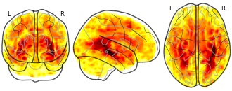
Collection description

Subject species

homo sapiens

Modality

Structural MRI

Cognitive paradigm (task)

None / Other

Map type

T

The extent to which the public takes an interest in politics has long been argued to be foundational to democracy, but the want of appropriate data has prevented cross-national and longitudinal analysis. This letter takes advantage of recent advances in latent-variable modeling of aggregate survey responses and a comprehensive collection of survey data to generate dynamic comparative estimates of macrointerest, that is, aggregate political interest, for over a hundred countries over the past four decades. These macrointerest scores are validated with other aggregate measures of political interest and of other types of political engagement. A cross-national and longitudinal analysis of macrointerest in advanced democracies reveals that along with election campaigns and inclusive institutions, it is good economic conditions, not bad times, that spur publics to greater interest in politics.

Context

The main idea behind this dataset was to get an idea on the Data collected and reported on COVID19 across the whole world along with the Timestamp. This dataset consolidates the COVID19 data reported globally along with Timestamp that can help future study on Time Series Analysis and Forecasting.

Content

It contains the combined, wrangled data reported in and around the world along with their Geographical Region including Latitudinal and Longitudinal Data, Time, along with the number of Confirmed Cases, Death Cases and Recovered Cases. Please note that the original data is reported and updated as per the Timeseries data on Confirmed Cases, Recovered Cases and Death Cases that gets updated from the JHU data repository on every 7 days. These separate Data Sources are next updated in Kaggle Notebook on every 15 days to 30 days.

Acknowledgements

The data is collected and compiled from John Hopkins University, "COVID-19 Data Repository by the Center for Systems Science and Engineering (CSSE) at Johns Hopkins University" or "JHU CSSE COVID-19 Data" for short and the url: https://github.com/CSSEGISandData/COVID-19. Johns Hopkins University, National Science Foundation (NSF), Bloomberg Philanthropies, Stavros Niarchos Foundation; Resource support: AWS, Slack, Github; Technical support: Johns Hopkins Applied Physics Lab (APL), Esri Living Atlas team, Kaggle Notebook.

Inspiration

Some great work to see would include, but not limited to: 1. Geographical Time Series Data Analysis 2. Time Series Analysis on Confirmed, Recovered and Death Cases 3. Forecasting on Geographical Area wise Cases Distribution

This dataset contains anonymized logs of user-level YouTube viewing activity, collected via Amazon Mechanical Turk. Each user in the dataset provided at least six months of their YouTube watch history, enabling longitudinal analysis of personal viewing patterns.

Each row in the dataset represents a single watch event and includes metadata such as: - the video ID - watch timestamp - whether the user was subscribed to the channel at the time - and whether the video was part of a playlist

This dataset is intended to support research in user behavior modeling, content recommendation systems, temporal video engagement, and personalized analytics.

The dataset accompanies the paper:

"A YouTube dataset with user-level usage data: Baseline characteristics and key insights"
Authors: Shruti Lall, Mohit Agarwal, Raghupathy Sivakumar
Conference: IEEE ICC 2020 – International Conference on Communications

If you use this dataset in your research, please cite the paper above.

Abstract copyright UK Data Service and data collection copyright owner.

Background
The Labour Force Survey (LFS) is a unique source of information using international definitions of employment and unemployment and economic inactivity, together with a wide range of related topics such as occupation, training, hours of work and personal characteristics of household members aged 16 years and over. It is used to inform social, economic and employment policy. The LFS was first conducted biennially from 1973-1983. Between 1984 and 1991 the survey was carried out annually and consisted of a quarterly survey conducted throughout the year and a 'boost' survey in the spring quarter (data were then collected seasonally). From 1992 quarterly data were made available, with a quarterly sample size approximately equivalent to that of the previous annual data. The survey then became known as the Quarterly Labour Force Survey (QLFS). From December 1994, data gathering for Northern Ireland moved to a full quarterly cycle to match the rest of the country, so the QLFS then covered the whole of the UK (though some additional annual Northern Ireland LFS datasets are also held at the UK Data Archive). Further information on the background to the QLFS may be found in the documentation.

Longitudinal data
The LFS retains each sample household for five consecutive quarters, with a fifth of the sample replaced each quarter. The main survey was designed to produce cross-sectional data, but the data on each individual have now been linked together to provide longitudinal information. The longitudinal data comprise two types of linked datasets, created using the weighting method to adjust for non-response bias. The two-quarter datasets link data from two consecutive waves, while the five-quarter datasets link across a whole year (for example January 2010 to March 2011 inclusive) and contain data from all five waves. A full series of longitudinal data has been produced, going back to winter 1992. Linking together records to create a longitudinal dimension can, for example, provide information on gross flows over time between different labour force categories (employed, unemployed and economically inactive). This will provide detail about people who have moved between the categories. Also, longitudinal information is useful in monitoring the effects of government policies and can be used to follow the subsequent activities and circumstances of people affected by specific policy initiatives, and to compare them with other groups in the population. There are however methodological problems which could distort the data resulting from this longitudinal linking. The ONS continues to research these issues and advises that the presentation of results should be carefully considered, and warnings should be included with outputs where necessary.

New reweighting policy
Following the new reweighting policy ONS has reviewed the latest population estimates made available during 2019 and have decided not to carry out a 2019 LFS and APS reweighting exercise. Therefore, the next reweighting exercise will take place in 2020. These will incorporate the 2019 Sub-National Population Projection data (published in May 2020) and 2019 Mid-Year Estimates (published in June 2020). It is expected that reweighted Labour Market aggregates and microdata will be published towards the end of 2020/early 2021.

LFS Documentation
The documentation available from the Archive to accompany LFS datasets largely consists of the latest version of each user guide volume alongside the appropriate questionnaire for the year concerned. However, volumes are updated periodically by ONS, so users are advised to check the latest documents on the ONS Labour Force Survey - User Guidance pages before commencing analysis. This is especially important for users of older QLFS studies, where information and guidance in the user guide documents may have changed over time.

Additional data derived from the QLFS
The Archive also holds further QLFS series: End User Licence (EUL) quarterly data; Secure Access datasets; household datasets; quarterly, annual and ad hoc module datasets compiled for Eurostat; and some additional annual Northern Ireland datasets.

Variables DISEA and LNGLST
Dataset A08 (Labour market status of disabled people) which ONS suspended due to an apparent discontinuity between April to June 2017 and July to September 2017 is now available. As a result of this apparent discontinuity and the inconclusive...