Histograms and results of k-means and Ward's clustering for Hidden Room game

The fileset contains information from three sources:

1. Histograms files:
* Lexical_histogram.png (histogram of lexical error ratios)
* Grammatical_histogram.png (histogram of grammatical error ratios)

2. K-means clustering files:
* elbow-lex kmeans.png (clustering by lexical aspects: error curves obtained for applying elbow method to determinate the optimal number of clusters)
* cube-lex kmeans.png (clustering by lexical aspects: a three-dimensional representation of clusters obtained after applying k-means method)
* Lexical_clusters (table) kmeans.xls (clustering by lexical aspects: centroids, standard deviations and number of instances assigned to each cluster)
* elbow-gram kmeans.png (clustering by grammatical aspects: error curves obtained for applying elbow method to determinate the optimal number of clusters)
* cube-gramm kmeans.png (clustering by grammatical aspects: a three-dimensional representation of clusters obtained after applying k-means method)
* Grammatical_clusters (table) kmeans.xls (clustering by grammatical aspects: centroids, standard deviations and number of instances assigned to each cluster)
* elbow-lexgram kmeans.png (clustering by lexical and grammatical aspects: error curves obtained for applying elbow method to determinate the optimal number of clusters)
* Lexical_Grammatical_clusters (table) kmeans.xls (clustering by lexical and grammatical aspects: centroids, standard deviations and number of instances assigned to each cluster)
* Grammatical_clusters_number_of_words (table) kmeans.xls : number of words (from column 2 to 4) and sizes (last column) obtained per each cluster by applying k-means clustering to grammatical error ratios.
* Lexical_clusters_number_of_words (table) kmeans.xls : number of words (from column 2 to 4) and sizes (last column) obtained per each cluster by applying k-means clustering to lexical error ratios.
* Lexical_Grammatical_clusters_number_of_words (table) kmeans.xls : number of words (from column 2 to 4) and sizes (last column) obtained per each cluster by applying k-means clustering to lexical and grammatical error ratios.

3. Ward’s Agglomerative Hierarchical Clustering files:
* Lexical_Cluster_Dendrogram_ward.png (clustering by lexical aspects: dendrogram obtained after applying Ward's clustering method).
* Grammatical_Cluster_Dendrogram_ward.png (clustering by grammatical aspects: dendrogram obtained after applying Ward's clustering method)
* Lexical_Grammatical_Cluster_Dendrogram_ward.png (clustering by lexical and grammatical aspects: dendrogram obtained after applying Ward's clustering method)
* Lexical_Grammatical_clusters (table) ward.xls: Centroids (from column 2 to 7) and cluster sizes (last column) obtained by applying Ward's agglomerative hierarchical clustering to lexical and grammatical error ratios.
* Grammatical_clusters (table) ward.xls: Centroids (from column 2 to 4) and cluster sizes (last column) obtained by applying Ward's agglomerative hierarchical clustering to grammatical error ratios.
* Lexical_clusters (table) ward.xls: Centroids (from column 2 to 4) and cluster sizes (last column) obtained by applying Ward's agglomerative hierarchical clustering to lexical error ratios.
* Lexical_clusters_number_of_words (table) ward.xls: number of words (from column 2 to 4) and sizes (last column) obtained per each cluster by applying Ward's agglomerative hierarchical clustering to lexical error ratios.
* Grammatical_clusters_number_of_words (table) ward.xls: number of words (from column 2 to 4) and sizes (last column) obtained per each cluster by applying Ward's agglomerative hierarchical clustering to grammatical error ratios.
* Lexical_Grammatical_clusters_number_of_words (table) ward.xls: number of words (from column 2 to 4) and sizes (last column) obtained per each cluster by applying Ward's agglomerative hierarchical clustering to lexical and grammatical error ratios.

The purpose of data mining analysis is always to find patterns of the data using certain kind of techiques such as classification or regression. It is not always feasible to apply classification algorithms directly to dataset. Before doing any work on the data, the data has to be pre-processed and this process normally involves feature selection and dimensionality reduction. We tried to use clustering as a way to reduce the dimension of the data and create new features. Based on our project, after using clustering prior to classification, the performance has not improved much. The reason why it has not improved could be the features we selected to perform clustering are not well suited for it. Because of the nature of the data, classification tasks are going to provide more information to work with in terms of improving knowledge and overall performance metrics. From the dimensionality reduction perspective: It is different from Principle Component Analysis which guarantees finding the best linear transformation that reduces the number of dimensions with a minimum loss of information. Using clusters as a technique of reducing the data dimension will lose a lot of information since clustering techniques are based a metric of 'distance'. At high dimensions euclidean distance loses pretty much all meaning. Therefore using clustering as a "Reducing" dimensionality by mapping data points to cluster numbers is not always good since you may lose almost all the information. From the creating new features perspective: Clustering analysis creates labels based on the patterns of the data, it brings uncertainties into the data. By using clustering prior to classification, the decision on the number of clusters will highly affect the performance of the clustering, then affect the performance of classification. If the part of features we use clustering techniques on is very suited for it, it might increase the overall performance on classification. For example, if the features we use k-means on are numerical and the dimension is small, the overall classification performance may be better. We did not lock in the clustering outputs using a random_state in the effort to see if they were stable. Our assumption was that if the results vary highly from run to run which they definitely did, maybe the data just does not cluster well with the methods selected at all. Basically, the ramification we saw was that our results are not much better than random when applying clustering to the data preprocessing. Finally, it is important to ensure a feedback loop is in place to continuously collect the same data in the same format from which the models were created. This feedback loop can be used to measure the model real world effectiveness and also to continue to revise the models from time to time as things change.

Background: Biomechanical studies of ACL injury risk factors frequently analyze only a fraction of the relevant data, and typically not in accordance with the injury mechanism. Extracting a peak value within a time series of relevance to ACL injuries is challenging due to differences in the relative timing and size of the peak value of interest.

Aims/hypotheses: The aim was to cluster analyze the knee valgus moment time series curve shape in the early stance phase. We hypothesized that 1a) There would be few discrete curve shapes, 1b) there would be a shape reflecting an early peak of the knee valgus moment, 2a) youth athletes of both sexes would show similar frequencies of early peaks, 2b) adolescent girls would have greater early peak frequencies.

Methods: N = 213 (39% boys) youth soccer and team handball athletes (phase 1) and N = 35 (45% boys) with 5 year follow-up data (phase 2) were recorded performing a change of direction task with 3D motion analysis and a force plate. The time series of the first 30% of stance phase were cluster analyzed based on Euclidean distances in two steps; shape-based main clusters with a transformed time series, and magnitude based sub-clusters with body weight normalized time series. Group differences (sex, phase) in curve shape frequencies, and shape-magnitude frequencies were tested with chi-squared tests.

Results: Six discrete shape-clusters and 14 magnitude based sub-clusters were formed. Phase 1 boys had greater frequency of early peaks than phase 1 girls (38% vs 25% respectively, P <  0.001 for full test). Phase 2 girls had greater frequency of early peaks than phase 2 boys (42% vs 21% respectively, P <  0.001 for full test).

Conclusions: Cluster analysis can reveal different patterns of curve shapes in biomechanical data, which likely reflect different movement strategies. The early peak shape is relatable to the ACL injury mechanism as the timing of its peak moment is consistent with the timing of injury. Greater frequency of early peaks demonstrated by Phase 2 girls is consistent with their higher risk of ACL injury in sports.

The Data Analytics Consulting Services market is experiencing robust growth, driven by the increasing adoption of data-driven decision-making across various industries. The market, estimated at $50 billion in 2025, is projected to exhibit a Compound Annual Growth Rate (CAGR) of 15% from 2025 to 2033, reaching approximately $150 billion by 2033. This expansion is fueled by several key factors: the proliferation of big data, advancements in artificial intelligence (AI) and machine learning (ML) technologies, and the rising need for businesses to gain actionable insights from their data to improve operational efficiency, enhance customer experience, and drive innovation. Key segments driving growth include predictive data analysis, used extensively for forecasting and risk management, and data mining, crucial for uncovering hidden patterns and trends within vast datasets. Large enterprises are the primary consumers of these services, investing heavily in advanced analytics to gain a competitive edge, followed by a rapidly growing segment of SMEs seeking to leverage data analytics for streamlined operations and improved decision-making. Significant regional variations are expected. North America, particularly the United States, is anticipated to maintain a substantial market share due to the presence of established technology giants and a mature data analytics ecosystem. However, regions like Asia-Pacific, especially India and China, are demonstrating rapid growth due to increasing digitalization and a burgeoning demand for data-driven solutions. While the market faces challenges such as data security concerns, the scarcity of skilled data scientists, and the high cost of implementation, the overall growth trajectory remains positive, driven by the undeniable value proposition of data analytics for businesses of all sizes and across various sectors. Competitive landscape is highly fragmented, with a mix of global consulting firms (Accenture, Deloitte, McKinsey), specialized data analytics companies (DataArt, Analytics8), and regional players competing for market share.

Promoters of genes associated with type 1 diabetes (T1D), Intermediary Diabetes Mellitus (IDM) and type 2 diabetes (T2D). T1D promoters (blue dots), T2D promoters (red dots) and promoters from genes associated with the “intermediary” phenotype (green dots).

DATA MINING THE GALAXY ZOO MERGERS STEVEN BAEHR, ARUN VEDACHALAM, KIRK BORNE, AND DANIEL SPONSELLER Abstract. Collisions between pairs of galaxies usually end in the coalescence (merger) of the two galaxies. Collisions and mergers are rare phenomena, yet they may signal the ultimate fate of most galaxies, including our own Milky Way. With the onset of massive collection of astronomical data, a computerized and automated method will be necessary for identifying those colliding galaxies worthy of more detailed study. This project researches methods to accomplish that goal. Astronomical data from the Sloan Digital Sky Survey (SDSS) and human-provided classifications on merger status from the Galaxy Zoo project are combined and processed with machine learning algorithms. The goal is to determine indicators of merger status based solely on discovering those automated pipeline-generated attributes in the astronomical database that correlate most strongly with the patterns identified through visual inspection by the Galaxy Zoo volunteers. In the end, we aim to provide a new and improved automated procedure for classification of collisions and mergers in future petascale astronomical sky surveys. Both information gain analysis (via the C4.5 decision tree algorithm) and cluster analysis (via the Davies-Bouldin Index) are explored as techniques for finding the strongest correlations between human-identified patterns and existing database attributes. Galaxy attributes measured in the SDSS green waveband images are found to represent the most influential of the attributes for correct classification of collisions and mergers. Only a nominal information gain is noted in this research, however, there is a clear indication of which attributes contribute so that a direction for further study is apparent.

These data sets were originally created for the following publications:

M. E. Houle, H.-P. Kriegel, P. Kröger, E. Schubert, A. Zimek
Can Shared-Neighbor Distances Defeat the Curse of Dimensionality?
In Proceedings of the 22nd International Conference on Scientific and Statistical Database Management (SSDBM), Heidelberg, Germany, 2010.

H.-P. Kriegel, E. Schubert, A. Zimek
Evaluation of Multiple Clustering Solutions
In 2nd MultiClust Workshop: Discovering, Summarizing and Using Multiple Clusterings Held in Conjunction with ECML PKDD 2011, Athens, Greece, 2011.

The outlier data set versions were introduced in:

E. Schubert, R. Wojdanowski, A. Zimek, H.-P. Kriegel
On Evaluation of Outlier Rankings and Outlier Scores
In Proceedings of the 12th SIAM International Conference on Data Mining (SDM), Anaheim, CA, 2012.

They are derived from the original image data available at https://aloi.science.uva.nl/

The image acquisition process is documented in the original ALOI work: J. M. Geusebroek, G. J. Burghouts, and A. W. M. Smeulders, The Amsterdam library of object images, Int. J. Comput. Vision, 61(1), 103-112, January, 2005

Additional information is available at: https://elki-project.github.io/datasets/multi_view

The following views are currently available:

Feature type	Description	Files
Object number	Sparse 1000 dimensional vectors that give the true object assignment	objs.arff.gz
RGB color histograms	Standard RGB color histograms (uniform binning)	aloi-8d.csv.gz aloi-27d.csv.gz aloi-64d.csv.gz aloi-125d.csv.gz aloi-216d.csv.gz aloi-343d.csv.gz aloi-512d.csv.gz aloi-729d.csv.gz aloi-1000d.csv.gz
HSV color histograms	Standard HSV/HSB color histograms in various binnings	aloi-hsb-2x2x2.csv.gz aloi-hsb-3x3x3.csv.gz aloi-hsb-4x4x4.csv.gz aloi-hsb-5x5x5.csv.gz aloi-hsb-6x6x6.csv.gz aloi-hsb-7x7x7.csv.gz aloi-hsb-7x2x2.csv.gz aloi-hsb-7x3x3.csv.gz aloi-hsb-14x3x3.csv.gz aloi-hsb-8x4x4.csv.gz aloi-hsb-9x5x5.csv.gz aloi-hsb-13x4x4.csv.gz aloi-hsb-14x5x5.csv.gz aloi-hsb-10x6x6.csv.gz aloi-hsb-14x6x6.csv.gz
Color similiarity	Average similarity to 77 reference colors (not histograms) 18 colors x 2 sat x 2 bri + 5 grey values (incl. white, black)	aloi-colorsim77.arff.gz (feature subsets are meaningful here, as these features are computed independently of each other)
Haralick features	First 13 Haralick features (radius 1 pixel)	aloi-haralick-1.csv.gz
Front to back	Vectors representing front face vs. back faces of individual objects	front.arff.gz
Basic light	Vectors indicating basic light situations	light.arff.gz
Manual annotations	Manually annotated object groups of semantically related objects such as cups	manual1.arff.gz

Outlier Detection Versions

Additionally, we generated a number of subsets for outlier detection:

Feature type	Description	Files
RGB Histograms	Downsampled to 100000 objects (553 outliers)	aloi-27d-100000-max10-tot553.csv.gz aloi-64d-100000-max10-tot553.csv.gz
	Downsampled to 75000 objects (717 outliers)	aloi-27d-75000-max4-tot717.csv.gz aloi-64d-75000-max4-tot717.csv.gz
	Downsampled to 50000 objects (1508 outliers)	aloi-27d-50000-max5-tot1508.csv.gz aloi-64d-50000-max5-tot1508.csv.gz

Summary descriptive statistics for cluster 2 for detection data from Barrow Island between 2009 and 2015.

The coronavirus disease 2019 pandemic has impacted and changed consumer behavior because of a prolonged quarantine and lockdown. This study proposed a theoretical framework to explore and define the influencing factors of online consumer purchasing behavior (OCPB) based on electronic word-of-mouth (e-WOM) data mining and analysis. Data pertaining to e-WOM were crawled from smartphone product reviews from the two most popular online shopping platforms in China, Jingdong.com and Taobao.com. Data processing aimed to filter noise and translate unstructured data from complex text reviews into structured data. The machine learning based K-means clustering method was utilized to cluster the influencing factors of OCPB. Comparing the clustering results and Kotler’s five products level, the influencing factors of OCPB were clustered around four categories: perceived emergency context, product, innovation, and function attributes. This study contributes to OCPB research by data mining and analysis that can adequately identify the influencing factors based on e-WOM. The definition and explanation of these categories may have important implications for both OCPB and e-commerce.

The size and share of the market is categorized based on Type (Data Mining, Predictive Data Analysis, Cluster Analysis, Data Summary, Others) and Application (SMEs, Large Enterprises) and geographical regions (North America, Europe, Asia-Pacific, South America, and Middle-East and Africa).

Anomaly detection is a process of identifying items, events or observations, which do not conform to an expected pattern in a dataset or time series. Current and future missions and our research communities challenge us to rapidly identify features and anomalies in complex and voluminous observations to further science and improve decision support. Given this data intensive reality, we propose to develop an anomaly detection system, called OceanXtremes, powered by an intelligent, elastic Cloud-based analytic service backend that enables execution of domain-specific, multi-scale anomaly and feature detection algorithms across the entire archive of ocean science datasets. A parallel analytics engine will be developed as the key computational and data-mining core of OceanXtreams' backend processing. This analytic engine will demonstrate three new technology ideas to provide rapid turn around on climatology computation and anomaly detection: 1. An adaption of the Hadoop/MapReduce framework for parallel data mining of science datasets, typically large 3 or 4 dimensional arrays packaged in NetCDF and HDF. 2. An algorithm profiling service to efficiently and cost-effectively scale up hybrid Cloud computing resources based on the needs of scheduled jobs (CPU, memory, network, and bursting from a private Cloud computing cluster to public cloud provider like Amazon Cloud services). 3. An extension to industry-standard search solutions (OpenSearch and Faceted search) to provide support for shared discovery and exploration of ocean phenomena and anomalies, along with unexpected correlations between key measured variables. We will use a hybrid Cloud compute cluster (private Eucalyptus on-premise at JPL with bursting to Amazon Web Services) as the operational backend. The key idea is that the parallel data-mining operations will be run 'near' the ocean data archives (a local 'network' hop) so that we can efficiently access the thousands of (say, daily) files making up a three decade time-series, and then cache key variables and pre-computed climatologies in a high-performance parallel database. OceanXtremes will be equipped with both web portal and web service interfaces for users and applications/systems to register and retrieve oceanographic anomalies data. By leveraging technology such as Datacasting (Bingham, et.al, 2007), users can also subscribe to anomaly or 'event' types of their interest and have newly computed anomaly metrics and other information delivered to them by metadata feeds packaged in standard Rich Site Summary (RSS) format. Upon receiving new feed entries, users can examine the metrics and download relevant variables, by simply clicking on a link, to begin further analyzing the event. The OceanXtremes web portal will allow users to define their own anomaly or feature types where continuous backend processing will be scheduled to populate the new user-defined anomaly type by executing the chosen data mining algorithm (i.e. differences from climatology or gradients above a specified threshold). Metadata on the identified anomalies will be cataloged including temporal and geospatial profiles, key physical metrics, related observational artifacts and other relevant metadata to facilitate discovery, extraction, and visualization. Products created by the anomaly detection algorithm will be made explorable and subsettable using Webification (Huang, et.al, 2014) and OPeNDAP (http://opendap.org) technologies. Using this platform scientists can efficiently search for anomalies or ocean phenomena, compute data metrics for events or over time-series of ocean variables, and efficiently find and access all of the data relevant to their study (and then download only that data).

Descriptive statistics (e.g., mean, median, standard deviation, percentile) of each variable extracted from Principal Component Analysis for each exercise cluster in elite professional female futsal players.

Intermetallics contribute significantly to our current demand for high-performance functional materials. However, understanding their chemistry is still an open and debated topic, especially for complex compounds such as approximants and quasicrystals. In this work, targeted topological data mining succeeded in (i) selecting all known Mackay-type approximants, (ii) uncovering the most important geometrical and chemical factors involved in their formation, and (iii) guiding the experimental work to obtain a new binary Sc–Pd 1/1 approximant for icosahedral quasicrystals containing the desired cluster. Single-crystal X-ray diffraction data analysis supplemented by electron density reconstruction using the maximum entropy method, showed fine structural peculiarities, that is, smeared electron densities in correspondence to some crystallographic sites. These characteristics have been studied through a comprehensive density functional theory modeling based on the combination of point defects such as vacancies and substitutions. It was confirmed that the structural disorder occurs in the shell enveloping the classical Mackay cluster, so that the real structure can be viewed as an assemblage of slightly different, locally ordered, four shell nanoclusters. Results obtained here open up broader perspectives for machine learning with the aim of designing novel materials in the fruitful field of quasicrystals and their approximants. This might become an alternative and/or complementary way to the electronic pseudogap tuning, often used before explorative synthesis.

This dataset provides comprehensive information on road intersection crashes involving public transport (Bus, Bus-train, Combi/minibusses, midibusses) recognised as "high-high" clusters within the City of Cape Town. It includes detailed records of all intersection crashes and their corresponding crash attribute combinations, which were prevalent in at least 10% of the total "high-high" cluster public transport road intersection crashes for the years 2017, 2018, 2019, and 2021.The dataset is meticulously organised according to support metric values, ranging from 0,10 to 0,171, with entries presented in descending order.Data SpecificsData Type: Geospatial-temporal categorical dataFile Format: Excel document (.xlsx)Size: 160 KBNumber of Files: The dataset contains a total of 1620 association rulesDate Created: 23rd May 2024MethodologyData Collection Method: The descriptive road traffic crash data per crash victim involved in the crashes was obtained from the City of Cape Town Network InformationSoftware: ArcGIS Pro, PythonProcessing Steps: Following the spatio-temporal analyses and the derivation of "high-high" cluster fishnet grid cells from a cluster and outlier analysis, all the road intersection crashes involving public transport that occurred within the "high-high" cluster fishnet grid cells were extracted to be processed by association analysis. The association analysis of these crashes was processed using Python software and involved the use of a 0,10 support metric value. Consequently, commonly occurring crash attributes among at least 10% of the "high-high" cluster road intersection public transport crashes were extracted for inclusion in this dataset.Geospatial InformationSpatial Coverage:West Bounding Coordinate: 18°20'EEast Bounding Coordinate: 19°05'ENorth Bounding Coordinate: 33°25'SSouth Bounding Coordinate: 34°25'SCoordinate System: South African Reference System (Lo19) using the Universal Transverse Mercator projectionTemporal InformationTemporal Coverage:Start Date: 01/01/2017End Date: 31/12/2021 (2020 data omitted)

D indicates the dataset containing N data objects, and its a priori partition with l categories is . The result obtained from clustering is , where k is the number of clusters. SS indicates that both objects belong to the same cluster of C and to the same group of partitions P; SD indicates points that belong to the same cluster of C and to different groups of P; DS indicates points that belong to different clusters of C and to the same group of P; and DD indicates points that belong to different clusters of C and to different groups of P.

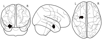
Connectivity-based parcellation (CBP) of the left human amygdala. Cluster #3 (blue) - laterobasal nuclei group

Collection description

We here employed methods for large-scale data mining to perform a connectivity-derived parcellation of the human amygdala based on whole-brain coactivation patterns computed for each seed voxel. Using this approach, connectivity-based parcellation divided the amygdala into three distinct clusters that are highly consistent with earlier microstructural distinctions. Meta-analytic connectivity modelling and functional characterization further revealed that the amygdala's laterobasal nuclei group was associated with coordinating high-level sensory input, whereas its centromedial nuclei group was linked to mediating attentional, vegetative, and motor responses. The results of this model-free approach support the concordance of structural, connectional, and functional organization in the human amygdala. This dataset was automatically imported from the ANIMA <http://anima.modelgui.org/> database. Version: 1

Subject species

homo sapiens

Modality

fMRI-BOLD

Analysis level

meta-analysis

Cognitive paradigm (task)

None / Other

Map type

M

This dataset provides comprehensive information on road intersection pedestrian crashes resulting in serious injuries and/or fatalities recognised as "high-high" clusters within the City of Cape Town. It includes detailed records of all intersection crashes and their corresponding crash attribute combinations, which were prevalent in at least 23% of the total "high-high" cluster pedestrian road intersection crashes resulting in serious injuries and/or fatalities for the years 2017, 2018 and 2019. The dataset is meticulously organised according to confidence metric values presented in descending order.Data SpecificsData Type: Geospatial-temporal categorical dataFile Format: Excel document (.xlsx)Size: 18,3 KBNumber of Files: The dataset contains a total of 258 association rulesDate Created: 24th May 2024MethodologyData Collection Method: The descriptive road traffic crash data per crash victim involved in the crashes was obtained from the City of Cape Town Network InformationSoftware: ArcGIS Pro, PythonProcessing Steps: Following the spatio-temporal analyses and the derivation of "high-high" cluster fishnet grid cells from a cluster and outlier analysis, all the road intersection pedestrian crashes resulting in serious injuries and/or fatalities that occurred within the "high-high" cluster fishnet grid cells were extracted to be processed by association analysis. The association analysis of these crashes was processed using Python software and involved the use of a 0,20 support metric value. Consequently, commonly occurring crash attributes among at least 20% of the "high-high" cluster road intersection pedestrian crashes resulting in serious injuries and/or fatalities were extracted for inclusion in this dataset.Geospatial InformationSpatial Coverage:West Bounding Coordinate: 18°20'EEast Bounding Coordinate: 19°05'ENorth Bounding Coordinate: 33°25'SSouth Bounding Coordinate: 34°25'SCoordinate System: South African Reference System (Lo19) using the Universal Transverse Mercator projectionTemporal InformationTemporal Coverage:Start Date: 01/01/2017End Date: 31/12/2019

Eight derived variables defined in the SAP (Cluster cardiovascular drugs, cluster cerebrovascular drugs, cluster cardiovascular diseases, cluster cerebrovascular diseases, cluster anti-hypertensive drugs, cluster anti-psychotic drugs, cluster anti-diabetic drugs, cluster lipid-lowering drugs) were included in each assessment, which yields 106 variables. The inclusion of TRT as a variable, which is implicit in our evaluation, gives 107 variables in total.Percent missing values were as follows: Testosterone (baseline), Free testosterone [18], % free testosterone, Bioavailable testosterone, % bioavailable testosterone = 79%; PSA (baseline) = 70%; Alcohol frequency = 38%; SHBG (baseline) = 33%; PGISS baseline, Previous overactive bladder therapy (Y/N) = 28%; Qmax, ED duration, ED aetiology, ED severity = 23%; IIEF baseline severity, IIEF-EF (baseline), IIEF-OF (baseline), IIEF-OS (baseline), IIEF-SD (baseline), IIEF-IS (baseline) = 14%; Albumin (baseline) = 2%; Renal impairment I, Renal impairment II, Renal impairment I (≥80), Renal impairment II (≥90) = 1%. prior α-blocking agents, β-blockers, calcium channels blockers, angiotensin converting enzyme inhibitors, angiotensin receptor blockers and diuretics.Baseline characteristics of the ITT population used for data mining analysis.

The retrieval of important information from a dataset requires applying a special data mining technique known as data clustering (DC). DC classifies similar objects into a groups of similar characteristics. Clustering involves grouping the data around k-cluster centres that typically are selected randomly. Recently, the issues behind DC have called for a search for an alternative solution. Recently, a nature-based optimization algorithm named Black Hole Algorithm (BHA) was developed to address the several well-known optimization problems. The BHA is a metaheuristic (population-based) that mimics the event around the natural phenomena of black holes, whereby an individual star represents the potential solutions revolving around the solution space. The original BHA algorithm showed better performance compared to other algorithms when applied to a benchmark dataset, despite its poor exploration capability. Hence, this paper presents a multi-population version of BHA as a generalization of the BHA called MBHA wherein the performance of the algorithm is not dependent on the best-found solution but a set of generated best solutions. The method formulated was subjected to testing using a set of nine widespread and popular benchmark test functions. The ensuing experimental outcomes indicated the highly precise results generated by the method compared to BHA and comparable algorithms in the study, as well as excellent robustness. Furthermore, the proposed MBHA achieved a high rate of convergence on six real datasets (collected from the UCL machine learning lab), making it suitable for DC problems. Lastly, the evaluations conclusively indicated the appropriateness of the proposed algorithm to resolve DC issues.

ACCESS THE INTERACTIVE MAP VIA RELATED URLS AT THE BOTTOM OF THIS RECORD Space-Time Pattern Mining for recorded depression prevalence from 2011 to 2022, based on the Anselin Local Moran’s I algorithm. The unit of analysis of this geospatial analysis was the Lower Super Output Area (LSOA). There are 32,844 LSOAs across England, with an average population of 1500 people (Office for National Statistics, 2021). In all analyses, we used the LSOA boundaries published by the Office for National Statistics as at March 21, 2021 (Office for National Statistics, 2021). The diagnosed depression prevalence was derived using the data published by NHS Digital. Figures showing the recorded prevalence of depression in England by general practitioner (GP) practice are published annually in the Quality and Outcomes Framework (QOF) administrative dataset, which also reports how the QOF-recorded prevalence has changed since the previous year (NHS Digital, 2020, pp. 2019–2020). For this study, we combined all available data on depression published by NHS Digital and created time-series recorded depression for each LSOA from 2011 to 2022. The annual aggregate data on diagnoses of depression per LSOA has been calculated based on the weighted averages of the number of patients diagnosed with depression per LSOA divided by the total number of registered patients in each LSOA. In terms of coverage, the data for Quality and Outcomes Framework (QOF) have been collected annually at an aggregate level for each of the 6470 (97.5%) GP practices in England, with approximately 61 million registered patients aged 18 years and above; thus, the dataset offers nationwide insights. This online app depicts interactively the Cluster and Outlier Analysis, using the Anselin Local Moran’s I algorithm (Anselin, 1995), to identify local indicators of spatial association (LISA) and correct for spatial dependence. The conceptualisation of spatial relationships parameter value was set as the ‘Contiguity edges corners’, the standardisation option was set as ‘Row’, and the number of permutations was set as 999. The LISA refer to statistically significant spatial clusters of small areas with high values (high/high clusters) and low values (low/low clusters) of depression, as well as high and low spatial outliers in which a high value is surrounded by low values (high/low clusters), and outliers in which a low value is surrounded by high values (low/high clusters).