- N
Connectivity-Based Parcellation of the Human Orbitofrontal Cortex: K=7...
- neurovault.org
niftiUpdated Nov 18, 2024+ more versions Share
Share Facebook
 Twitter
 EmailClick to copy linkLink copiedCite(2024). Connectivity-Based Parcellation of the Human Orbitofrontal Cortex: K=7 cluster map [Dataset]. http://identifiers.org/neurovault.image:887628niftiAvailable download formatsUnique identifierhttps://identifiers.org/neurovault.image:887628Dataset updatedNov 18, 2024License
CC0 1.0 Universal Public Domain Dedicationhttps://creativecommons.org/publicdomain/zero/1.0/
License information was derived automaticallyDescriptionK=7 cluster map based on N=13 participants.
Collection description
K-means cluster maps of orbitofrontal cortex with K=2, 3, 4, 5, 6, and 7 clusters based on resting-state fMRI data.
Subject species
homo sapiens
Modality
fMRI-BOLD
Analysis level
group
Cognitive paradigm (task)
rest eyes open
Map type
R
Canadian Cluster Map Portal Data
- open.canada.ca
csvUpdated Feb 21, 2022+ more versionsShareFacebookTwitterEmailClick to copy linkLink copiedCiteInnovation, Science and Economic Development Canada (2022). Canadian Cluster Map Portal Data [Dataset]. https://open.canada.ca/data/en/dataset/83c19800-74a9-4da5-8d67-d2e0611e167fcsvAvailable download formatsDataset updatedFeb 21, 2022LicenseOpen Government Licence - Canada 2.0https://open.canada.ca/en/open-government-licence-canada
License information was derived automaticallyTime period coveredJan 1, 2006 - Dec 31, 2017Area coveredCanadaDescriptionThe datasets provided encompass all the statistics found on the Canadian Cluster Map Portal. Moreover, additional information such as cluster-concordance and cluster descriptions are provided to allow for accurate analysis of the data.
R script and datasets - Cluster Analysis and Heat maps
- figshare.com
txtUpdated May 30, 2020ShareFacebookTwitterEmailClick to copy linkLink copiedCiteChui Pin Leaw; Po Teen Lim; Li Keat Lee (2020). R script and datasets - Cluster Analysis and Heat maps [Dataset]. http://doi.org/10.6084/m9.figshare.12387242.v2txtAvailable download formatsUnique identifierhttps://doi.org/10.6084/m9.figshare.12387242.v2Dataset updatedMay 30, 2020Dataset provided byfigshareAuthorsChui Pin Leaw; Po Teen Lim; Li Keat LeeLicenseAttribution 4.0 (CC BY 4.0)https://creativecommons.org/licenses/by/4.0/
License information was derived automaticallyDescriptionThis folder contained R scripts and data sets used to generate clustering dendogram and heatmaps as shown Fig. 3.
Indicative Flood Risk Areas - Clusters
- environment.data.gov.uk
Updated Jan 20, 2017+ more versionsShareFacebookTwitterEmailClick to copy linkLink copiedCiteEnvironment Agency (2017). Indicative Flood Risk Areas - Clusters [Dataset]. https://environment.data.gov.uk/dataset/27325bdc-dbfd-4d10-bdb7-b0298703d082Dataset updatedJan 20, 2017LicenseOpen Government Licence 3.0http://www.nationalarchives.gov.uk/doc/open-government-licence/version/3/
License information was derived automaticallyDescriptionPLEASE NOTE: this dataset has been retired. It has been superseded by data for Flood Risk Areas: https://environment.data.gov.uk/dataset/f3d63ec5-a21a-49fb-803a-0fa0fb7238b6
The Indicative Flood Risk Areas are primarily based on an aggregated 1km square grid Updated Flood Map for Surface Water (1 in 100 and 1000 annual probability rainfall), informally referred to as the “blue square map”.
• Cluster Maps – are aggregations of 3km by 3km squares that each contain at least 4 (in Wales) or 5 (in England) touching "blue squares" (i.e. 1km grid squares where one of the thresholds above is exceeded)
This dataset forms part of Indicative Flood Risk Areas (shapefiles)
A bundle download of all Indicative Flood Risk Areas spatial datasets is also available from this record. Please see individual records for full details and metadata on each product.
- f
World Clusters map
- data.apps.fao.org
ShareFacebookTwitterEmailClick to copy linkLink copiedCiteWorld Clusters map [Dataset]. https://data.apps.fao.org/map/catalog/static/search?createDateYear=1995Area coveredWorldDescriptionWorld cluster map of the world based on a Coastal zone (LOICZ) database received in 1995 from the Netherlands Institute for Sea Research (NIOZ).
Links to all datasets and downloads for 80 A0/A3 digital image of map...
- researchdata.edu.au
- data.csiro.au
datadownloadUpdated Jan 18, 2016+ more versionsShareFacebookTwitterEmailClick to copy linkLink copiedCiteSuzanne Prober; Tom Harwood; Nat Raisbeck-Brown; Kristen Williams (2016). Links to all datasets and downloads for 80 A0/A3 digital image of map posters accompanying AdaptNRM Guide: Helping Biodiversity Adapt: supporting climate adaptation planning using a community-level modelling approach [Dataset]. https://researchdata.edu.au/653610/653610datadownloadAvailable download formatsDataset updatedJan 18, 2016AuthorsSuzanne Prober; Tom Harwood; Nat Raisbeck-Brown; Kristen WilliamsLicensehttps://research.csiro.au/dap/licences/csiro-data-licence/https://research.csiro.au/dap/licences/csiro-data-licence/
Time period coveredJan 1, 2015 - Jan 10, 2015Area coveredDescriptionThis dataset is a series of digital map-posters accompanying the AdaptNRM Guide: Helping Biodiversity Adapt: supporting climate adaptation planning using a community-level modelling approach.
These represent supporting materials and information about the community-level biodiversity models applied to climate change. Map posters are organised by four biological groups (vascular plants, mammals, reptiles and amphibians), two climate change scenario (1990-2050 MIROC5 and CanESM2 for RCP8.5), and five measures of change in biodiversity.
The map-posters present the nationally consistent data at locally relevant resolutions in eight parts – representing broad groupings of NRM regions based on the cluster boundaries used for climate adaptation planning (http://www.environment.gov.au/climate-change/adaptation) and also Nationally.
Map-posters are provided in PNG image format at moderate resolution (300dpi) to suit A0 printing. The posters were designed to meet A0 print size and digital viewing resolution of map detail. An additional set in PDF image format has been created for ease of download for initial exploration and printing on A3 paper. Some text elements and map features may be fuzzy at this resolution.
Each map-poster contains four dataset images coloured using standard legends encompassing the potential range of the measure, even if that range is not represented in the dataset itself or across the map extent.
Most map series are provided in two parts: part 1 shows the two climate scenarios for vascular plants and mammals and part 2 shows reptiles and amphibians. Eight cluster maps for each series have a different colour theme and map extent. A national series is also provided. Annotation briefly outlines the topics presented in the Guide so that each poster stands alone for quick reference.
An additional 77 National maps presenting the probability distributions of each of 77 vegetation types – NVIS 4.1 major vegetation subgroups (NVIS subgroups) - are currently in preparation.
Example citations:
Williams KJ, Raisbeck-Brown N, Prober S, Harwood T (2015) Generalised projected distribution of vegetation types – NVIS 4.1 major vegetation subgroups (1990 and 2050), A0 map-poster 8.1 - East Coast NRM regions. CSIRO Land and Water Flagship, Canberra. Available online at www.AdaptNRM.org and https://data.csiro.au/dap/.
Williams KJ, Raisbeck-Brown N, Harwood T, Prober S (2015) Revegetation benefit (cleared natural areas) for vascular plants and mammals (1990-2050), A0 map-poster 9.1 - East Coast NRM regions. CSIRO Land and Water Flagship, Canberra. Available online at www.AdaptNRM.org and https://data.csiro.au/dap/.
This dataset has been delivered incrementally. Please check that you are accessing the latest version of the dataset. Lineage: The map posters show case the scientific data. The data layers have been developed at approximately 250m resolution (9 second) across the Australian continent to incorporate the interaction between climate and topography, and are best viewed using a geographic information system (GIS). Each data layers is 1Gb, and inaccessible to non-GIS users. The map posters provide easy access to the scientific data, enabling the outputs to be viewed at high resolution with geographical context information provided.
Maps were generated using layout and drawing tools in ArcGIS 10.2.2
A check list of map posters and datasets is provided with the collection.
Map Series: 7.(1-77) National probability distribution of vegetation type – NVIS 4.1 major vegetation subgroup pre-1750 #0x
8.1 Generalised projected distribution of vegetation types (NVIS subgroups) (1990 and 2050)
9.1 Revegetation benefit (cleared natural areas) for plants and mammals (1990-2050)
9.2 Revegetation benefit (cleared natural areas) for reptiles and amphibians (1990-2050)
10.1 Need for assisted dispersal for vascular plants and mammals (1990-2050)
10.2 Need for assisted dispersal for reptiles and amphibians (1990-2050)
11.1 Refugial potential for vascular plants and mammals (1990-2050)
11.1 Refugial potential for reptiles and amphibians (1990-2050)
12.1 Climate-driven future revegetation benefit for vascular plants and mammals (1990-2050)
12.2 Climate-driven future revegetation benefit for vascular reptiles and amphibians (1990-2050)
- d
Database for the geologic map of the central San Juan caldera cluster,...
- datasets.ai
- catalog.data.gov
55Updated Oct 8, 2024ShareFacebookTwitterEmailClick to copy linkLink copiedCiteDepartment of the Interior (2024). Database for the geologic map of the central San Juan caldera cluster, southwestern Colorado [Dataset]. https://datasets.ai/datasets/database-for-the-geologic-map-of-the-central-san-juan-caldera-cluster-southwestern-colorad55Available download formatsDataset updatedOct 8, 2024Dataset authored and provided byDepartment of the InteriorArea coveredColoradoDescriptionThis geodatabase contains all the geologic map information for the Geologic Map of the San Juan caldera cluster, southwestern Colorado and is part of U.S. Geological Survey Geologic Investigations Map Series I-2799. The San Juan Mountains are the largest erosional remnant of a composite volcanic field that covered much of the southern Rocky Mountains in middle Tertiary time. The San Juan field consists mainly of intermediate-composition lavas and breccias, erupted about 35-30 Ma from scattered central volcanoes (Conejos Formation) and overlain by voluminous ash-flow sheets erupted from caldera sources. In the central San Juan Mountains, eruption of at least 8,800 km3 of dacitic-rhyolitic magma as nine major ash flow sheets (individually 150-5,000 km3) was accompanied by recurrent caldera subsidence between 28.3 Ma and about 26.5 Ma. Voluminous andesitic-dacitic lavas and breccias were erupted from central volcanoes prior to the ash-flow eruptions, and similar lava eruptions continued within and adjacent to the calderas during the period of more silicic explosive volcanism. Exposed calderas vary in size from 10 to 75 km in maximum dimension, the largest calderas being associated with the most voluminous eruptions.
- U
Database for the Geologic Map of the Katmai Volcanic Cluster, Katmai...
- data.usgs.gov
- datasets.ai
- +1more
Updated Aug 27, 2024+ more versionsShareFacebookTwitterEmailClick to copy linkLink copiedCiteJeff Peters; Joel Robinson; David Ramsey; Tracey Felger; Edward Hildreth; Judith Fierstein (2024). Database for the Geologic Map of the Katmai Volcanic Cluster, Katmai National Park, Alaska [Dataset]. http://doi.org/10.5066/P9K3XRENUnique identifierhttps://doi.org/10.5066/P9K3XRENDataset updatedAug 27, 2024AuthorsJeff Peters; Joel Robinson; David Ramsey; Tracey Felger; Edward Hildreth; Judith FiersteinLicenseU.S. Government Workshttps://www.usa.gov/government-works
License information was derived automaticallyTime period covered1996 - 2001Area coveredAlaskaDescriptionA database of the geologic map of the Katmai Volcanic Cluster as described in the original abstract: This digital publication contains all the geologic map information used to publish U.S. Geological Survey Geologic Investigations Map Series I-2778 (Hildreth and Fierstein, 2003). This is a geologic map of the Katmai volcanic cluster on the Alaska Peninsula (including Mount Katmai, Trident Volcano, Mount Mageik, Mount Martin, Mount Griggs, Snowy Mountain, Alagogshak volcano, and Novarupta volcano), and shows the distribution of ejecta from the great eruption of June, 1912 at Novarupta. Widely scattered erosional remnants of volcanic rocks, unrelated to but in the vicinity of the Katmai cluster, are also mapped. Distribution of glacial deposits, large landslides, debris avalanches, and surficial deposits are a snapshot of an ever-changing landscape.
- e
Indicative Flood Risk Areas - Clusters
- data.europa.eu
- cloud.csiss.gmu.edu
unknownUpdated Jun 16, 2021ShareFacebookTwitterEmailClick to copy linkLink copiedCiteEnvironment Agency (2021). Indicative Flood Risk Areas - Clusters [Dataset]. https://data.europa.eu/data/datasets/indicative-flood-risk-areas-clusters?locale=ptunknownAvailable download formatsDataset updatedJun 16, 2021Dataset authored and provided byEnvironment AgencyLicenseOpen Government Licence 3.0http://www.nationalarchives.gov.uk/doc/open-government-licence/version/3/
License information was derived automaticallyDescriptionThe Indicative Flood Risk Areas are primarily based on an aggregated 1km square grid Updated Flood Map for Surface Water (1 in 100 and 1000 annual probability rainfall), informally referred to as the “blue square map”.
• Cluster Maps – are aggregations of 3km by 3km squares that each contain at least 4 (in Wales) or 5 (in England) touching "blue squares" (i.e. 1km grid squares where one of the thresholds above is exceeded)
This dataset forms part of Indicative Flood Risk Areas (shapefiles)
A bundle download of all Indicative Flood Risk Areas spatial datasets is also available from this record. Please see individual records for full details and metadata on each product. Attribution statement: © Environment Agency copyright and/or database right 2016. All rights reserved.
- d
Neighborhood Clusters
- catalog.data.gov
- opendata.dc.gov
Updated Feb 5, 2025+ more versionsShareFacebookTwitterEmailClick to copy linkLink copiedCiteD.C. Office of the Chief Technology Officer (2025). Neighborhood Clusters [Dataset]. https://catalog.data.gov/dataset/neighborhood-clustersDataset updatedFeb 5, 2025Dataset provided byD.C. Office of the Chief Technology OfficerDescriptionThis data set describes Neighborhood Clusters that have been used for community planning and related purposes in the District of Columbia for many years. It does not represent boundaries of District of Columbia neighborhoods. Cluster boundaries were established in the early 2000s based on the professional judgment of the staff of the Office of Planning as reasonably descriptive units of the City for planning purposes. Once created, these boundaries have been maintained unchanged to facilitate comparisons over time, and have been used by many city agencies and outside analysts for this purpose. (The exception is that 7 “additional” areas were added to fill the gaps in the original dataset, which omitted areas without significant neighborhood character such as Rock Creek Park, the National Mall, and the Naval Observatory.) The District of Columbia does not have official neighborhood boundaries. The Office of Planning provides a separate data layer containing Neighborhood Labels that it uses to place neighborhood names on its maps. No formal set of standards describes which neighborhoods are included in that dataset.Whereas neighborhood boundaries can be subjective and fluid over time, these Neighborhood Clusters represent a stable set of boundaries that can be used to describe conditions within the District of Columbia over time.
- a
Cluster Commercial Development District
- data-cityoflynchburg.opendata.arcgis.com
- data.virginia.gov
- +1more
Updated May 31, 2016ShareFacebookTwitterEmailClick to copy linkLink copiedCiteCity of Lynchburg (2016). Cluster Commercial Development District [Dataset]. https://data-cityoflynchburg.opendata.arcgis.com/datasets/cluster-commercial-development-district/dataDataset updatedMay 31, 2016Dataset authored and provided byCity of LynchburgArea coveredDescriptionBoundary designating the Cluster Commercial Development District within the City of Lynchburg.
- a
Data from: Rural Cluster
- hub.arcgis.com
Updated Dec 29, 2015ShareFacebookTwitterEmailClick to copy linkLink copiedCiteAlachua County Board of County Commissioners (2015). Rural Cluster [Dataset]. https://hub.arcgis.com/maps/acgm::rural-clusterDataset updatedDec 29, 2015Dataset authored and provided byAlachua County Board of County CommissionersArea coveredDescriptionFuture Land Use Map for Alachua County, Fl
Hydrochemical Clusters Map: K-Means Clustering Results for Southcentral...
- figshare.com
htmlUpdated Jan 11, 2025ShareFacebookTwitterEmailClick to copy linkLink copiedCiteAbhinav Choudhary (2025). Hydrochemical Clusters Map: K-Means Clustering Results for Southcentral Alaska [Dataset]. http://doi.org/10.6084/m9.figshare.28188833.v1htmlAvailable download formatsUnique identifierhttps://doi.org/10.6084/m9.figshare.28188833.v1Dataset updatedJan 11, 2025AuthorsAbhinav ChoudharyLicenseAttribution 4.0 (CC BY 4.0)https://creativecommons.org/licenses/by/4.0/
License information was derived automaticallyArea coveredSouthcentral Alaska, AlaskaDescriptionThis interactive map shows the spatial distribution of hydrochemical data across Southcentral Alaska using K-Means clustering. The dataset includes key hydrochemical measurements, and each cluster is represented by a unique color on the map. The map is generated using Leaflet and Folium libraries in Python.The static version is available in the main manuscript, while this HTML file provides a dynamic exploration of clustering results.Contact: Abhinav Choudhary (Chandigarh University, MSc Data Science)Date of creation: 2025-01-11
- d
Maps from the M2-ACT survey for point sources in tSZ-Selected Galaxy...
- search.dataone.org
Updated Sep 24, 2024ShareFacebookTwitterEmailClick to copy linkLink copiedCiteDICKER, SIMON (2024). Maps from the M2-ACT survey for point sources in tSZ-Selected Galaxy Clusters. [Dataset]. http://doi.org/10.7910/DVN/FQNKYXUnique identifierhttps://doi.org/10.7910/DVN/FQNKYXDataset updatedSep 24, 2024Dataset provided byHarvard DataverseAuthorsDICKER, SIMONDescriptionUsing MUSTANG2 on the Green Bank Telescope a survey at 90GHz was carried out searching for point sources in Galaxy Clusters from the ACT DR5 data release. The survey was designed to characterize the population of sources that could affect the measured Sunyaev-Zel'dovich Effect signal by experiments such as ACT and has an angular resolution of 10" and a 5 sigma sensitivity of ~1mJy. We provide raw and filtered maps for each cluster in fits format.
- a
School Cluster Boundaries (MCPS) (File Geodatabase)
- hub.arcgis.com
- data-mcplanning.hub.arcgis.com
Updated Jun 1, 2023+ more versionsShareFacebookTwitterEmailClick to copy linkLink copiedCiteMontgomery Maps (2023). School Cluster Boundaries (MCPS) (File Geodatabase) [Dataset]. https://hub.arcgis.com/datasets/577d81c6fd6049a69fcf17a12f4e6449Dataset updatedJun 1, 2023Dataset authored and provided byMontgomery MapsLicenseMIT Licensehttps://opensource.org/licenses/MIT
License information was derived automaticallyArea coveredMontgomery County Public SchoolsDescriptionGroups of geographically defined attendance areas. They include elementary and middle-level schools that feed into particular high schools and consortium schools.For further details: https://www2.montgomeryschoolsmd.org/departments/Clusteradmin/Clusters/indexFor more information, contact: GIS Manager Information Technology & Innovation (ITI) Montgomery County Planning Department, MNCPPC T: 301-650-5620
- H
Clustering of Ncloud maps
- dataverse.harvard.edu
Updated Oct 4, 2021ShareFacebookTwitterEmailClick to copy linkLink copiedCiteGiuseppe Puglisi (2021). Clustering of Ncloud maps [Dataset]. http://doi.org/10.7910/DVN/XAMJ4XCroissantCroissant is a format for machine-learning datasets. Learn more about this at mlcommons.org/croissant.Unique identifierhttps://doi.org/10.7910/DVN/XAMJ4XDataset updatedOct 4, 2021Dataset provided byHarvard DataverseAuthorsGiuseppe PuglisiLicenseCC0 1.0 Universal Public Domain Dedicationhttps://creativecommons.org/publicdomain/zero/1.0/
License information was derived automaticallyDescriptionHealpix maps of Nclouds from https://iopscience.iop.org/article/10.3847/1538-4357/abb6f5 and the uncertainties Map of patches estimated from spectral clustering .
Cluster descriptions.
- plos.figshare.com
xlsUpdated Nov 30, 2023+ more versionsShareFacebookTwitterEmailClick to copy linkLink copiedCiteWaad R. Alolayan; Jana M. Rieger; Minn N. Yoon (2023). Cluster descriptions. [Dataset]. http://doi.org/10.1371/journal.pone.0294712.t002xlsAvailable download formatsUnique identifierhttps://doi.org/10.1371/journal.pone.0294712.t002Dataset updatedNov 30, 2023AuthorsWaad R. Alolayan; Jana M. Rieger; Minn N. YoonLicenseAttribution 4.0 (CC BY 4.0)https://creativecommons.org/licenses/by/4.0/
License information was derived automaticallyDescriptionWith the increasing focus on patient-centred care, this study sought to understand priorities considered by patients and healthcare providers from their experience with head and neck cancer treatment, and to compare how patients’ priorities compare to healthcare providers’ priorities. Group concept mapping was used to actively identify priorities from participants (patients and healthcare providers) in two phases. In phase one, participants brainstormed statements reflecting considerations related to their experience with head and neck cancer treatment. In phase two, statements were sorted based on their similarity in theme and rated in terms of their priority. Multidimensional scaling and cluster analysis were performed to produce multidimensional maps to visualize the findings. Two-hundred fifty statements were generated by participants in the brainstorming phase, finalized to 94 statements that were included in phase two. From the sorting activity, a two-dimensional map with stress value of 0.2213 was generated, and eight clusters were created to encompass all statements. Timely care, education, and person-centred care were the highest rated priorities for patients and healthcare providers. Overall, there was a strong correlation between patient and healthcare providers’ ratings (r = 0.80). Our findings support the complexity of the treatment planning process in head and neck cancer, evident by the complex maps and highly interconnected statements related to the experience of treatment. Implications for improving the quality of care delivered and care experience of head and cancer are discussed.
- u
Canadian Cluster Map Portal Data - Catalogue - Canadian Urban Data Catalogue...
- data.urbandatacentre.ca
- beta.data.urbandatacentre.ca
Updated Oct 1, 2024ShareFacebookTwitterEmailClick to copy linkLink copiedCite(2024). Canadian Cluster Map Portal Data - Catalogue - Canadian Urban Data Catalogue (CUDC) [Dataset]. https://data.urbandatacentre.ca/dataset/gov-canada-83c19800-74a9-4da5-8d67-d2e0611e167fDataset updatedOct 1, 2024LicenseOpen Government Licence - Canada 2.0https://open.canada.ca/en/open-government-licence-canada
License information was derived automaticallyArea coveredCanadaDescriptionThe datasets provided encompass all the statistics found on the Canadian Cluster Map Portal. Moreover, additional information such as cluster-concordance and cluster descriptions are provided to allow for accurate analysis of the data.
- M
School Clusters Map
- data.montgomeryschoolsmd.org
application/rdfxml +5Updated Jun 23, 2016ShareFacebookTwitterEmailClick to copy linkLink copiedCite(2016). School Clusters Map [Dataset]. https://data.montgomeryschoolsmd.org/widgets/cmed-dzx8?mobile_redirect=truecsv, tsv, application/rdfxml, application/rssxml, json, xmlAvailable download formatsDataset updatedJun 23, 2016DescriptionMCPS Cluster Service Areas
- g
Physical Clustering of the World's Oceans | gimi9.com
- gimi9.com
Updated Jul 31, 2018+ more versionsShareFacebookTwitterEmailClick to copy linkLink copiedCite(2018). Physical Clustering of the World's Oceans | gimi9.com [Dataset]. https://gimi9.com/dataset/au_physical-clustering-of-the-worlds-oceansDataset updatedJul 31, 2018Area coveredWorldDescriptionPhysical Clustering of the World's Oceans (based on data extracted from World Ocean Atlas 2013 version 2). Data. The physical regions are based on the observations of the World Ocean Atlas 2013 version 2 (WOA13v2*; https://www.nodc.noaa.gov/OC5/woa13/). We extracted the decadal annual means for nine variables. These variables included: Temperature (°C), Salinity (unitless), Density (kg/m3), Dissolved Oxygen (ml/l), Apparent Oxygen Utilization (ml/l), Silicate (µmol/l), Phosphate (µmol/l), Density (kg/m^3) and Nitrate (µmol/l). The datasets for Temperature, Salinity and Dissolved oxygen were provided at 0.25° resolution. We therefore reprojected the remaining WOA13v2 datasets to the same projection by making each 1° cell in these datasets at 0.25° resolution, while assigning the original value to the four finer resolution cells. For the seafloor physical regions we included two additional dataset derived from GEBCO bathymetry data (https://www.gebco.net/). The first dataset was the bathymetry across the seafloor, this layer was re-projected to 0.25° resolution, were the cell values were based on the mean values of the finer scale GEBCO layer. We then computed the slope of depth based on the bathymetry raster using the ‘terrain’ function in the ‘raster’ package. Analysis. We generated physical clusters for the globe at the surface (0m), 200m, 1000m and the seafloor. For the surface, 200m and 1000m regions, we extracted the single depth layers from the WOA13v2 datasets and generated a matrix which represented the sites by the variables. For the seafloor, we had to generate interpolated layers at the seafloor based on the WOA13v2 data. We did this by looking at the mean depth of the bathymetry data and undertaking a tri-linear (cubic) interpolation of the WOA13v2 data at that seafloor depth. We subsequently ran a tri-linear interpolation of the WOA13v2 for each variable and generated maps of seafloor environmental conditions. One these maps were generated we extracted each variable into a seafloor site by seafloor physical variable matrix. All four site by physical variables datasets (0, 200, 1000 and seafloor) were then scaled in an attempt to centre and normalise the data. For each of these four datasets we then fitted a k-means clustering model from 2 to 40 clusters and looked at the resulting model loglikelihood, AIC and BIC. We then selected the number of clusters at the point were the the log-likelihood converged (i.e. the point were additional centroids only gave a marginal increase in log-likelihood). The resulting cluster identity was then assigned to each site and used to generate maps of the physical clusters for each dataset. These rasters were then converted to shapefiles. Boyer, T.P., J. I. Antonov, O. K. Baranova, C. Coleman, H. E. Garcia, A. Grodsky, D. R. Johnson, R. A. Locarnini, A. V. Mishonov, T.D. O'Brien, C.R. Paver, J.R. Reagan, D. Seidov, I. V. Smolyar, and M. M. Zweng, 2013: World Ocean Database 2013, NOAA Atlas NESDIS 72, S. Levitus, Ed., A. Mishonov, Technical Ed.; Silver Spring, MD, 209 pp., http://doi.org/10.7289/V5NZ85MT
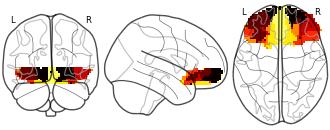
FacebookTwitterConnectivity-Based Parcellation of the Human Orbitofrontal Cortex: K=7 cluster map
CC0 1.0 Universal Public Domain Dedicationhttps://creativecommons.org/publicdomain/zero/1.0/
License information was derived automatically
K=7 cluster map based on N=13 participants.
Collection description
K-means cluster maps of orbitofrontal cortex with K=2, 3, 4, 5, 6, and 7 clusters based on resting-state fMRI data.
Subject species
homo sapiens
Modality
fMRI-BOLD
Analysis level
group
Cognitive paradigm (task)
rest eyes open
Map type
R