The Iris dataset was used in R.A. Fisher's classic 1936 paper, The Use of Multiple Measurements in Taxonomic Problems, and can also be found on the UCI Machine Learning Repository.

It includes three iris species with 50 samples each as well as some properties about each flower. One flower species is linearly separable from the other two, but the other two are not linearly separable from each other.

The columns in this dataset are:

• Id
• SepalLengthCm
• SepalWidthCm
• PetalLengthCm
• PetalWidthCm
• Species

This is perhaps the best known database to be found in the pattern recognition literature. Fisher's paper is a classic in the field and is referenced frequently to this day. (See Duda & Hart, for example.) The data set contains 3 classes of 50 instances each, where each class refers to a type of iris plant. One class is linearly separable from the other 2; the latter are NOT linearly separable from each other.

To use this dataset:

import tensorflow_datasets as tfds

ds = tfds.load('iris', split='train')
for ex in ds.take(4):
 print(ex)

See the guide for more informations on tensorflow_datasets.

Dataset

This dataset was created by sadaf koondhar

Contents

The "Iris Flower Visualization using Python" project is a data science project that focuses on exploring and visualizing the famous Iris flower dataset. The Iris dataset is a well-known dataset in the field of machine learning and data science, containing measurements of four features (sepal length, sepal width, petal length, and petal width) for three different species of Iris flowers (Setosa, Versicolor, and Virginica).

In this project, Python is used as the primary programming language along with popular libraries such as pandas, matplotlib, seaborn, and plotly. The project aims to provide a comprehensive visual analysis of the Iris dataset, allowing users to gain insights into the relationships between the different features and the distinct characteristics of each Iris species.

The project begins by loading the Iris dataset into a pandas DataFrame, followed by data preprocessing and cleaning if necessary. Various visualization techniques are then applied to showcase the dataset's characteristics and patterns. The project includes the following visualizations:

1. Scatter Plot: Visualizes the relationship between two features, such as sepal length and sepal width, using points on a 2D plane. Different species are represented by different colors or markers, allowing for easy differentiation.

2. Pair Plot: Displays pairwise relationships between all features in the dataset. This matrix of scatter plots provides a quick overview of the relationships and distributions of the features.

3. Andrews Curves: Represents each sample as a curve, with the shape of the curve representing the corresponding Iris species. This visualization technique allows for the identification of distinct patterns and separability between species.

4. Parallel Coordinates: Plots each feature on a separate vertical axis and connects the values for each data sample using lines. This visualization technique helps in understanding the relative importance and range of each feature for different species.

5. 3D Scatter Plot: Creates a 3D plot with three features represented on the x, y, and z axes. This visualization allows for a more comprehensive understanding of the relationships between multiple features simultaneously.

Throughout the project, appropriate labels, titles, and color schemes are used to enhance the visualizations' interpretability. The interactive nature of some visualizations, such as the 3D Scatter Plot, allows users to rotate and zoom in on the plot for a more detailed examination.

The "Iris Flower Visualization using Python" project serves as an excellent example of how data visualization techniques can be applied to gain insights and understand the characteristics of a dataset. It provides a foundation for further analysis and exploration of the Iris dataset or similar datasets in the field of data science and machine learning.

Dataset

This dataset was created by Hamza Tanç

Contents

A simple web page containing Fisher's Iris Dataset.

The Iris dataset is a classic and widely used dataset in machine learning for classification tasks. It consists of measurements of different iris flowers, including sepal length, sepal width, petal length, and petal width, along with their corresponding species. With a total of 150 samples, the dataset is balanced and serves as an excellent choice for understanding and implementing classification algorithms. This notebook explores the dataset, preprocesses the data, builds a decision tree classification model, and evaluates its performance, showcasing the effectiveness of decision trees in solving classification problems.

Iris dataset from open source.

Why this Dataset

This dataset brings to you Iris Dataset in several data formats (see more details in the next sections).

You can use it to test the ingestion of data in all these formats using Python or R libraries. We also prepared Python Jupyter Notebook and R Markdown report that input all these formats:

• Test Data Formats in Python
• Test Data Formats in R

Iris Dataset

Iris Dataset was created by R. A. Fisher and donated by Michael Marshall.

Repository on UCI site: https://archive.ics.uci.edu/ml/datasets/iris

Data Source: https://archive.ics.uci.edu/ml/machine-learning-databases/iris/

The file downloaded is iris.data and is formatted as a comma delimited file.

This small data collection was created to help you test your skills with ingesting various data formats.

Content

This file was processed to convert the data in the following formats: * csv - comma separated values format * tsv - tab separated values format * parquet - parquet format
* feather - feather format * parquet.gzip - compressed parquet format * h5 - hdf5 format * pickle - Python binary object file - pickle format * xslx - Excel format
* npy - Numpy (Python library) binary format * npz - Numpy (Python library) binary compressed format * rds - Rds (R specific data format) binary format

Acknowledgements

I would like to acknowledge the work of the creator of the dataset - R. A. Fisher and of the donor - Michael Marshall.

Inspiration

Use these data formats to test your skills in ingesting data in various formats.

Here we use Python to visualize how certain machine learning algorithms classify certain data points in the Iris dataset. Let's begin by importing the Iris dataset and splitting it into features and labels. We will use only the petal length and width for this analysis.

Dataset

This dataset was created by Anjali Wani

Contents

Palmer Penguins

The Palmer penguins dataset by Allison Horst, Alison Hill, and Kristen Gorman was first made publicly available as an R package. The goal of the Palmer Penguins dataset is to replace the highly overused Iris dataset for data exploration & visualization. However, now you can use Palmer penguins on Kaggle!

https://www.googleapis.com/download/storage/v1/b/kaggle-user-content/o/inbox%2F19186184%2Fa750e19f13e9c199fb47106d741e3b35%2FPalmerPenguins.png?generation=1720255432637209&alt=media" alt="Palmer Penguins">

License

Data are available by CC-0 license in accordance with the Palmer Station LTER Data Policy and the LTER Data Access Policy for Type I data.

Bibliography

Gorman KB, Williams TD, Fraser WR (2014) Ecological Sexual Dimorphism and Environmental Variability within a Community of Antarctic Penguins (Genus Pygoscelis). PLoS ONE 9(3): e90081. https://doi.org/10.1371/journal.pone.0090081

See also:

More information about the dataset is available in its official documentation.

The Palmer penguins dataset in Python: https://github.com/mcnakhaee/palmerpenguins/ The Palmer penguins dataset in Julia: https://github.com/devmotion/PalmerPenguins.jl

Source

https://huggingface.co/datasets/SIH/palmer-penguins

Dataset

This dataset was created by Mohan Pradhan

Released under Apache 2.0

Contents

This repository contains our raw datasets from channel measurements performed at the University of Utah campus. In addition, we have included a document that explains the setup and methodology used to collect this data, as well as a very brief discussion of results. File organization: * documentation/ - Contains a .docx with the description of the setup and evaluation. * data/ - HDF5 files containing both metadata and raw IQ samples for each location at which data was collected. Notice we collected data at 14 different client locations. See map in the attached docx (skipped locations 12 and 16). We deployed 5 different receivers at 5 different rooftops. Due to resource constraints, one set of files contains data from 4 different locations whereas another set contains information from the single remaining location.

We have developed a set of python scripts that allow us to parse and analyze the data. Although not included here, they can be found in our public repository: https://github.com/renew-wireless/RENEWLab You can find the top script here.

For more information on the POWDER-RENEW project please visit the POWDER website. The RENEW part of the project focuses on the deployment of an open-source massive MIMO system. Please visit our website for more information.

Successful Short-Term Volcanic Eruption Forecasting Using Seismic Features, Suplementary Material by Rey-Devesa (1,2), Benítez (3), Prudencio, Ligdamis Gutiérrez (1,2), Cortés (1,2), Titos (3), Koulakov (4,5), Zuccarello (6) and Ibáñez (1,2).
Institutions associated: (1) Department of Theoretical Physics and Cosmos. Science Faculty. Avd. Fuentenueva s/n. University of Granada. 18071. Granada. Spain. (2) Andalusian Institute of Geophysiscs. Campus de Cartuja. University of Granada. C/Profesor Clavera 12. 18071. Granada. Spain. (3) Department of Signal Theory, Telematics and Communication. University of Granada. Informatics and Telecommunication School. 18071. Granada. Spain. (4) Trofimuk Institute of Petroleum Geology and Geophysics SB RAS, Prospekt Koptyuga, 3, 630090 Novosibirsk, Russia (5) Institute of the Earth’s Crust SB RAS, Lermontova 128, Irkutsk, Russia (6) Istituto Nazionale di Geofisica e Vulcanologia, Sezione di Pisa (INGV-Pisa), via Cesare Battisti, 53, 56125, Pisa, Italy.
Acknowledgment: This study was partially supported by the Spanish FEMALE project (PID2019-106260GB-I00).
P. Rey-Devesa was funded by the Ministerio de Ciencia e Innovación del Gobierno de España (MCIN),
Agencia Estatal de Investigación (AEI), Fondo Social Europeo (FSE),
and Programa Estatal de Promoción del Talento y su Empleabilidad en I+D+I Ayudas para contratos predoctorales para la formación de doctores 2020 (PRE2020-092719).
Ivan Koulakov was supported by the Russian Science Foundation (Grant No. 20-17-00075).
Luciano Zuccarello was supported by the INGV Pianeta Dinamico 2021 Tema 8 SOME project (grant no. CUP D53J1900017001)
funded by the Italian Ministry of University and Research
“Fondo finalizzato al rilancio degli investimenti delle amministrazioni centrali dello Stato e allo sviluppo del Paese, legge 145/2018”.
English language editing was performed by Tornillo Scientific, UK.
Data availability statement: 1.- Seismic data from Kilauea, Augustine, Bezymianny (2007), and Mount St. Helens are available from the IRIS data repository (http://ds.iris.edu/seismon/index.phtml).
(An example of the Python code to access the data is described below.)
2.- Seismic data from Bezymianny (2017-2018) are available from Ivan Koulakov (ivan.science@gmail.com) upon request.
3.- Seismic data from Mt. Etna are available from INGV-Italy upon request (http://terremoti.ingv.it/en/help),
also available from the Zenodo data repository (https://doi.org/10.5281/zenodo.6849621). Access code in Python to download the records of Kilauea, Augustine and Mount St. Helens volcanoes, from the IRIS data repository. '''To access the raw signals please first install ObsPy and then execute following commands in a python console: ''' Example: from obspy.core import UTCDateTime
from obspy.clients.fdsn import Client
import obspy.io.mseed
client = Client('IRIS')
t1 = UTCDateTime('2006-01-10T00:00:00')
t2 = UTCDateTime('2006-01-12T00:00:00')
raw_data = client.get_waveforms(
network='AV',
station='AUH',
location='',
channel='HHZ',
starttime=t1,
endtime=t2) '''To further download station information execute: ''' xml = client.get_stations(network='AV',station='AUH',
channel='HHZ',starttime=t1,endtime=t2,level='response') ''' 'To scale the data using the station’s meta-data: ''' data = raw_data.remove_response(inventory=xml) ''' To filter, trim and plot the data execute: ''' data.write("Augustine.mseed", format="MSEED") data.filter('bandpass',freqmin=1.0,freqmax=20)
data.trim(t1+60,t2-60)
data.plot() Contents: 6 different Matlab codes. The principal code is called FeatureExtraction.
The codes rsac.m and ReadMSEEDFast.m are for reading different format of data. (Not developed by the group)
Seismic Data from Mt. Etna for using as an example.

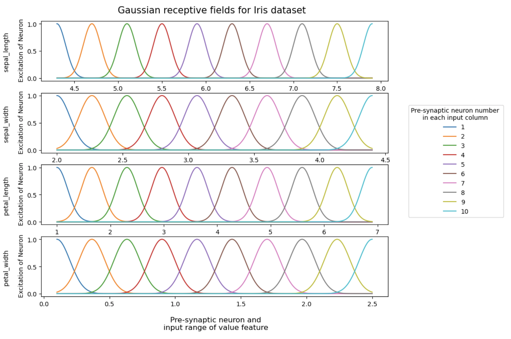
The classic iris dataset was encoded using Gaussian receptive fields for use in spiking neural networks. All transformations were done without using ready-made solutions related to SNN. Only NumPy and the sources provided at the end were used.
The classic dataset contains three types of flowers: Versicolor, Setosa, and Virginica.
Each class has 4 features: "Sepal Length", "Sepal Width", "Petal Length", and "Petal Width".
We will encode the values of each feature using the spike generation moments of 10 presynaptic neurons, resulting in a total of 40 presynaptic neurons.

Below, I will provide detailed Python code that encodes the data:

import pandas as pd
import numpy as np
import matplotlib.pyplot as plt
from scipy.stats import norm
import warnings
warnings.filterwarnings("ignore")

Load the original dataset from any convenient source: ``` URL =
'https://gist.githubusercontent.com/curran/a08a1080b88344b0c8a7/raw/0e7a9b0a5d22642a06d3d5b9bcbad9890c8ee534/iris.csv'

df = pd.read_csv(URL) Look at the first few lines of the dataset: df.head() ``` https://www.googleapis.com/download/storage/v1/b/kaggle-user-content/o/inbox%2F9529600%2F57f95917ff4b0eb8664996f405f0269c%2F2023-06-09%20%2000.10.56.png?generation=1686258722100757&alt=media" alt="">

Make a copy of the dataframe, delete the 'species' column, leaving only the quantitative part of the detaset: df_ = df.drop(columns=['species']).copy() Build a data histogram: df_.plot.hist(alpha=0.4, figsize=(20, 8)) plt.legend(title = "Dataset cilumns:" ,bbox_to_anchor = (1.0, 0.6), loc = 'upper left') plt.title('Iris dataset', fontsize = 20) plt.xlabel('Input value', fontsize = 15) plt.show() https://www.googleapis.com/download/storage/v1/b/kaggle-user-content/o/inbox%2F9529600%2Fea7374d10e92a7af57588f009f60e2a4%2F2023-06-09%20%2000.14.03.png?generation=1686258859622250&alt=media" alt=""> The data is distributed fairly evenly, which is why we will encode each feature with the 10 presynaptic neurons with same size, resulting in a total of 10 x 4 = 40 presynaptic neurons.

Let's write a function that generates 10 Gaussians for each input feature so that: - means of each Gaussian are evenly distributed between the extreme values of the range, including the boundaries for each feature ( "Sepal Length", "Sepal Width", "Petal Length", and "Petal Width"); - the height of each Gaussian is equal to 1 is the maximum excitation value of the presynaptic neuron, from which late we will calculate the spike generation latency by presynaptic neuron.

def Gaus_neuron(df, n, step, s):
  
  neurons_list = list()
  x_axis_list = list()
  t = 0
  
  for col in df.columns:
    
    vol = df[col].values
    min_ = np.min(vol)
    max_ = np.max(vol)
    x_axis = np.arange(min_, max_, step)
    x_axis[0] = min_
    x_axis[-1] = max_
    x_axis_list.append(np.round(x_axis, 10))
    neurons = np.zeros((n, len(x_axis)))
    
    for i in range(n):
      
      loc = (max_ - min_) * (i /(n-1)) + min_
      neurons[i] = norm.pdf(x_axis, loc, s[t])
      neurons[i] = neurons[i] / np.max(neurons[i])

    neurons_list.append(neurons)
    t += 1
  
  return neurons_list, x_axis_list

Select the parameters for uniform coverage of the range of possible values of each feature by Gaussians and apply the function written above: sigm = [0.1, 0.1, 0.2, 0.1] d = Gaus_neuron(df_, 10, 0.001, sigm) Now visualize Gaussians for our dataset for each input feature: ``` fig, (ax1, ax2, ax3, ax4) = plt.subplots(4)

fig.set_figheight(8) fig.set_figwidth(10)

k = 0

for ax in [ax1, ax2, ax3, ax4]:

ax.set(ylabel = f'{df_.columns[k]} 

Excitation of Neuron')

for i in range(len(d[0][k])):

  ax.plot(d[1][k], d[0][k][i], label = i + 1)

k+=1

plt.legend(title = "Presynaptic neuron number in each input column" ,bbox_to_anchor = (1.05, 3.25), loc = 'upper left') plt.suptitle('

Gaussian receptive fields for Iris dataset', fontsize = 15) ax.set_xlabel(' Presynaptic neurons and input range of value feature', fontsize = 12, labelpad = 15)

plt.show() ![](https://www.googleapis.com/download/storage/v1/b/kaggle-user-content/o/inbox%2F9529600%2F111954e059469c7522adb140b98101ca%2F2023-06-09%20%2015.48.10.png?generation=1686314920537433&alt=media) Now let's examine the encoding logic in detail using the first five data points of the "sepal_width" feature as an example: We will draw dotted vertical segments for the first five values of the "sepal_width" feature and locate their intersections with the Gaussian presynaptic neurons. These points will be marked with red dots: x_input = 5 fig, ax = plt.subplots(1)

fig.set_figheight(5) fi...

The EarthScope DS Noise Toolkit is a collection of 3 open-source Python script bundles for:

Computing Power Spectral Densities (PSD) of waveform data

Performing microseism energy computations from PSDs

Performing frequency dependent polarization analysis of seismograms

✓ https://cdnjs.cloudflare.com/ajax/libs/font-awesome/6.5.1/css/all.min.css">The Noise Toolkit code is available from the "EarthScope Noise Toolkit (NTK) GitHub repository":https://github.com/iris-edu/noise-toolkit.

Two UK Earth System Model (UKESM1) hindcasts have been performed in support of the Virtual Integration of Satellite and In-situ Observation Networks (VISION) project (NE/Z503393/1).

Data is provided as raw model output in Met Office PP (32-bit) format that can be read by the Iris (https://scitools-iris.readthedocs.io/en/stable/) or cf-python (https://ncas-cms.github.io/cf-python/) libraries.

This is global data at N96 L85 resolution (1.875 x 1.25, 85 model levels up to 85km). Simulations were performed on the Monsoon2 High Performance Computer (HPC).

The first dataset (Jan 1982 to May 2022) contains hourly ozone concentrations on the lowest model level (20m above the surface).

The second dataset (Jan 2010 to Dec 2020) contains hourly ozone concentrations and hourly Heaviside function on 37 fixed pressure levels. Data is only provided for days in which ozone was measured by the FAAM aircraft (for comparison purposes).

Ozone data is provided in mass mixing ratio (kg species/kg air).

Description: - This dataset includes all 22 built-in datasets from the Seaborn library, a widely used Python data visualization tool. Seaborn's built-in datasets are essential resources for anyone interested in practicing data analysis, visualization, and machine learning. They span a wide range of topics, from classic datasets like the Iris flower classification to real-world data such as Titanic survival records and diamond characteristics.

• Included Datasets:
  • Anagrams: Analysis of word anagram patterns.
  • Anscombe: Anscombe's quartet demonstrating the importance of data visualization.
  • Attention: Data on attention span variations in different scenarios.
  • Brain Networks: Connectivity data within brain networks.
  • Car Crashes: US car crash statistics.
  • Diamonds: Data on diamond properties including price, cut, and clarity.
  • Dots: Randomly generated data for scatter plot visualization.
  • Dow Jones: Historical records of the Dow Jones Industrial Average.
  • Exercise: The relationship between exercise and health metrics.
  • Flights: Monthly passenger numbers on flights.
  • FMRI: Functional MRI data capturing brain activity.
  • Geyser: Eruption times of the Old Faithful geyser.
  • Glue: Strength of glue under different conditions.
  • Health Expenditure: Health expenditure statistics across countries.
  • Iris: Famous dataset for classifying Iris species.
  • MPG: Miles per gallon for various vehicles.
  • Penguins: Data on penguin species and their features.
  • Planets: Characteristics of discovered exoplanets.
  • Sea Ice: Measurements of sea ice extent.
  • Taxis: Taxi trips data in a city.
  • Tips: Tipping data collected from a restaurant.
  • Titanic: Survival data from the Titanic disaster.

This complete collection serves as an excellent starting point for anyone looking to improve their data science skills, offering a wide array of datasets suitable for both beginners and advanced users.

Context

While working on money counter feature on our solution for helping the visually Impaired. after searching online we found out that there's no public dataset for Egyptian Currencies. We started by collecting dataset ourselves by taking pictures and labelling it. it was time consuming task. So we used Image synthesis techniques via OpenCV and Python. we wanted our dataset to exist in a variety of conditions such as different brightness. In the background we used Places365 dataset to have a realistic image

We will use this data for our solution in OpenCV AI Competition 2021. https://opencv.org/wp-content/uploads/2020/11/opencv-competition-1.jpg">

In the spirit of the Competition we decided to make our annotated dataset open-source to benefit the community so anyone who needs an Egyptian currencies dataset can start developing their solutions right away

Content

Dataset consists of 10k Images all are 1080*1080 you can easily resize it before training. dataset is annotated using Pascal Visual Object Classes(VOC) as an XML file. each 1000 images are loaded to a separate file for more freedom while splitting the train/test/val data.

The dataset were created randomly so no count for each class. Classes: 5, 10, 20, 50, 100, 200 https://i.pinimg.com/564x/e0/eb/25/e0eb25b5c76d026afaf47f65411bd921.jpg">

Acknowledgements

Competition: OpenCV AI Competition Inspired by : Playing card dataset generation video Playing card dataset generation repo Background : Places365 dataset