Logical Observation Identifiers Names and Codes (LOINC) is a database and universal standard for identifying medical laboratory observations. This dataset shows the codes which maps to source organization. Mapping each entity-specific code to its corresponding universal code can represent a significant investment of both human and financial capital.

The files linked to this reference are the geospatial data created as part of the completion of the baseline vegetation inventory project for the NPS park unit. Current format is ArcGIS file geodatabase but older formats may exist as shapefiles. In order to avoid two repetitive ground field efforts, the sampling plan was devised from a combination of both vegetation maps. Using OR logic, overlays were created using both maps as input for each class, and random samples were developed for each class in excess of 30 polygons. Where there were less than 30 polygons sample sites were selected non-randomly from each polygon (i.e. a 100% sample). A total of 512 ground sampling sites were developed from a total of 21 vegetation and land cover classes which are represented on both vegetation maps. Using GIS tools, an ASCII file was generated with ground coordinates representing each of these sites. The 512 sets of coordinates were appropriately re-formatted and directly downloaded as waypoints in three North American Rockwell PLGR GPS receivers. During the week of August 4, 1997 three field crews of two persons each worked together at the monument in a coordinated effort to identify vegetation/cover types at each of the sites. The field crews had a paper map showing the location of the plots and the polygon boundaries (but not attributes) overlaid on topographic data. One team member operated the GPS receiver to navigate to the site, and the other identified the vegetation/cover type and provided a general physical description of the site environs. Sites were considered to be circular with a radius of 50 m. from the coordinate point. Where 2 or more vegetation/cover types occurred, or there was a mosaic of types, all were described within the 50 m. radius of the site coordinate.

This data package shows the information of Logical Observation Identifiers Names Codes Map to Source Organization, Codes Source Organization and Names and Codes.

ABSTRACT Knowledge of the spatial variability of soil attributes is an aid to soil management. The aim of this study was to apply fuzzy logic and geostatistics in defining the spatial variability of soil fertility, in soil cultivated with the rubber tree. Soil samples from the 0-0.20 m and 0.20-0.40 m layers were collected in a stratified random sampling grid, with a shortest distance of 6 m, for a total of 60 points. The chemical attributes were P, K, Ca, Mg, BS, CEC and V. The spatial dependence of the attributes was determined, and the maps were constructed using ordinary kriging interpolation. The interpolated values were transformed into degrees of pertinence (FI), with the lower and upper limits previously defined, using an increasing model. The nutrient P displayed values in both layers below the recommended lower limit (< 20 mg dm-3). The rules of inference indicated that the total area shown in the fuzzy maps of soil fertility requires the application of correctives and fertiliser, as it has an FI < 0.50 and a percentage area > 50%. This methodology reduced the number of maps for interpreting soil fertility in the area, enabling visualisation of the spatial and gradual variability of the needs of the region.

Environmental Sensitivity Index (ESI) maps are an integral component in oil-spill contingency planning and assessment. They serve as a source of information in the event of an oil spill incident. ESI maps are a product of the Hazardous Materials Response Division of the Office of Response and Restoration (OR&R).ESI maps contain three types of information: shoreline habitats (classified according to their sensitivity to oiling), human-use resources, and sensitive biological resources. Most often, this information is plotted on 7.5 minute USGS quadrangles, although in Alaska, USGS topographic maps at scales of 1:63,360 and 1:250,000 are used, and in other atlases, NOAA charts have been used as the base map. Collections of these maps, grouped by state or a logical geographic area, are published as ESI atlases. Digital data have been published for most of the U.S. shoreline, including Alaska, Hawaii and Puerto Rico.

The HYDRO1k data sets are the result of the cooperative project at the U.S. Geological Survey's (U.S.G.S.) EROS Center. The goal of the project is the development of a globally consistent hydrologic derivative data set. The effort has been led by U.S.G.S. scientists in collaboration with the United Nations Environment Programme/Global Resource Information Database (UNEP/GRID) located in Sioux Falls, South Dakota.

Development of the HYDRO1k database was made possible by the completion of the 30 arc-second digital elevation model at EROS in 1996, entitled GTOPO30. This data set, with its nominal cell size of 1 km, has been and will continue to be applied by many scientists and researchers to hydrologic and land form studies. Inevitably, these studies require development, at a minimum, of a standard suite of derivative products. The HYDRO1k package provides, for each continent, a suite of six raster and two vector data sets. These data sets cover many of the common derivative products used in hydrologic analysis. The raster data sets are the hydrologically correct DEM, derived flow directions, flow accumulations, slope, aspect, and a compound topographic (wetness) index. The derived streamlines and basins are distributed as vector data sets.

Predictive understanding of cell signaling network operation based on general prior knowledge but consistent with empirical data in a specific environmental context is a current challenge in computational biology. Recent work has demonstrated that Boolean logic can be used to create context-specific network models by training proteomic pathway maps to dedicated biochemical data; however, the Boolean formalism is restricted to characterizing protein species as either fully active or inactive. To advance beyond this limitation, we propose a novel form of fuzzy logic sufficiently flexible to model quantitative data but also sufficiently simple to efficiently construct models by training pathway maps on dedicated experimental measurements. Our new approach, termed constrained fuzzy logic (cFL), converts a prior knowledge network (obtained from literature or interactome databases) into a computable model that describes graded values of protein activation across multiple pathways. We train a cFL-converted network to experimental data describing hepatocytic protein activation by inflammatory cytokines and demonstrate the application of the resultant trained models for three important purposes: (a) generating experimentally testable biological hypotheses concerning pathway crosstalk, (b) establishing capability for quantitative prediction of protein activity, and (c) prediction and understanding of the cytokine release phenotypic response. Our methodology systematically and quantitatively trains a protein pathway map summarizing curated literature to context-specific biochemical data. This process generates a computable model yielding successful prediction of new test data and offering biological insight into complex datasets that are difficult to fully analyze by intuition alone.

BackgroundThe use of implementation science in health research continues to increase, generating interest amongst those new to the field. However, conventional biomedical and health services research training does not necessarily equip scholars to incorporate theory-driven implementation science into their projects. Those new to IS may therefore struggle to apply abstract concepts from theory to their own work. In our teaching, we addressed this challenge by creating a practical teaching tool based on lessons from implementation mapping and the implementation research logic model (IRLM).The GUIDEThe tool is inspired by implementation mapping, the Implementation Research Logic Model, the ERIC implementation strategies, and Proctor's Outcomes Framework amongst other innumerable lessons from our experience as implementation scientists. We included sections to prompt learners to articulate the evidence-based practice of interest (including core and adaptable components) and the evidence-practice gap. The Guided Understanding of Implementation, Development & Education—GUIDE—and its corresponding prompts may provide a useful teaching tool to guide new users on incorporating implementation science into their evaluations. It also may help instructors illustrate how related implementation science concepts relate to each other over successive lessons or class sessions.ConclusionThis tool was developed from our experiences in teaching implementation science courses and consultation with new users in conjunction with common practices in the field including implementation mapping and the IRLM.

ABSTRACT Cacao is a species of great economic and social importance. Expanding the area grown with this crop has been limited by its climatic requirements. Agroclimatic zoning for agricultural sector and creation of land suitability maps by fuzzy logic contribute to such production expansion. In this sense, this study aimed to develop rainfall zoning for cacao in Bahia state using the fuzzy logic method. The used data came from rainfall historical series of 519 meteorological stations distributed throughout the state. Geostatistical analyses were used to quantify the spatial dependence degree of studied variable and kriging was used to develop maps representing mean monthly rainfall. These maps were submitted to continuous classification by fuzzy mapping for identification of high-risk areas for cocoa growing based on rainfall. Based on the fuzzy method, the southern mesoregion of Bahia state presented the highest rainfall uniformity, suggesting that this area is more suitable for cocoa growing.

In addition to displaying earthquakes by magnitude, this service also provide earthquake impact details. Impact is measured by population as well as models for economic and fatality loss. For more details, see: PAGER Alerts. Consumption Best Practices:As a service that is subject to very high usage, ensure peak performance and accessibility of your maps and apps by avoiding the use of non-cache-able relative Date/Time field filters. To accommodate filtering events by Date/Time, we suggest using the included "Age" fields that maintain the number of days or hours since a record was created or last modified, compared to the last service update. These queries fully support the ability to cache a response, allowing common query results to be efficiently provided to users in a high demand service environment.When ingesting this service in your applications, avoid using POST requests whenever possible. These requests can compromise performance and scalability during periods of high usage because they too are not cache-able. Update Frequency: Events are updated as frequently as every 5 minutes and are available up to 30 days with the following exceptions:Events with a Magnitude LESS than 4.5 are retained for 7 daysEvents with a Significance value, "sig" field, of 600 or higher are retained for 90 days In addition to event points, ShakeMaps are also provided. These have been dissolved by Shake Intensity to reduce the Layer Complexity.The specific layers provided in this service have been Time Enabled and include:Events by Magnitude: The event’s seismic magnitude value.Contains PAGER Alert Level: USGS PAGER (Prompt Assessment of Global Earthquakes for Response) system provides an automated impact level assignment that estimates fatality and economic loss.Contains Significance Level: An event’s significance is determined by factors like magnitude, max MMI, ‘felt’ reports, and estimated impact.Shake Intensity: The Instrumental Intensity or Modified Mercalli Intensity (MMI) for available events. For field terms and technical details, see: ComCat Documentation Alternate SymbologiesVisit the Classic USGS Feature Layer item for a Rainbow view of Shakemap features. RevisionsSep 16, 2025: Exposed ‘UniqueId’ field in Shake Intensity Polygon layer.Sep 14, 2025: Upgrade to Layer data update workflow, to improve reliability and scalability.Aug 14, 2024: Added a default Minimum scale suppression of 1:6,000,000 on Shake Intensity layer. Jul 11, 2024: Updated event popup, setting "Tsunami Warning" text to "Alert Possible" when flag is present. Also included hyperlink to tsunami warning center. Feb 13, 2024: Updated feed logic to remove Superseded events This map is provided for informational purposes and is not monitored 24/7 for accuracy and currency. Always refer to USGS source for official guidance. If you would like to be alerted to potential issues or simply see when this Service will update next, please visit our Live Feed Status Page!

Here we share the dataset set for the study titled "Flood Susceptibility Mapping using Fuzzy Analytical Hierarchy Process for Cedar Rapids, Iowa". Brief description and the data sources are provided for researchers. This dataset includes various demographic and geophysical features for the case study presented in the article below for the city of Cedar Rapids, Iowa.

• Elevation: Digital representation of the earth. Elevation is also called as DEM (Digital Elevation Model) Source: Iowa Department of Natural Resources
• River Drainage Density: The measurement of the total length of channels per unit area. Source: Generated using the river network data
• Soil Type: Soil type distribution over the region. Source: United States Department of Agriculture, Soil Survey Geographic Database
• Land use: Representation of land management over the region (i.e., urbanized, agricultural. pasture). Source: United States Department of Agriculture, CropScape and Cropland Data Layer
• Slope: The measurement of steepness of the region. Source: Generated using DEM
• Population: Number of inhabitants over the region. Source: Federal Emergency Management Agency, HAZUS Database
• Road Network Density: The measurement of the total length of road per unit area. Source: Generated using the transportation network
• Children & Elderly Population: Number of children and people over 65 years old over the region. Source: Federal Emergency Management Agency, HAZUS Database
• Renters: Number of renters over the region. Source: Federal Emergency Management Agency, HAZUS Database
• Income Rating: Income distribution over the region. Source: Federal Emergency Management Agency, HAZUS Database
• River Network: Geolocation of river bodies over the region. Source: Iowa Department of Natural Resources
• Transportation Network: Geolocation of vehicle roads over the region. Source: OpenStreetMap Vector Layers

Article: Cikmaz, B.A., Yildirim, E. and Demir, I., 2022. 'Flood susceptibility mapping using fuzzy analytical hierarchy process for Cedar Rapids, Iowa.', EarthArxiv, 3416. https://doi.org/10.31223/X57344"

Decades of research have revealed the remarkable complexity of the midbrain dopamine (DA) system, which comprises cells principally located in the ventral tegmental area (VTA) and substantia nigra pars compacta (SNc). Neither homogenous nor serving a singular function, the midbrain DA system is instead composed of distinct cell populations that (1) receive different sets of inputs, (2) project to separate forebrain sites, and (3) are characterized by unique transcriptional and physiological signatures. To appreciate how these differences relate to circuit function, we first need to understand the anatomical connectivity of unique DA pathways and how this connectivity relates to DA-dependent motivated behavior. We and others have provided detailed maps of the input-output relationships of several subpopulations of midbrain DA cells and explored the roles of these different cell populations in directing behavioral output. In this study, we analyze VTA inputs and outputs as a high dimensional dataset (10 outputs, 22 inputs), deploying computational techniques well-suited to finding interpretable patterns in such data. In addition to reinforcing our previous conclusion that the connectivity in the VTA is dependent on spatial organization, our analysis also uncovered a set of inputs elevated onto each projection-defined VTADA cell type. For example, VTADA→NAcLat cells receive preferential innervation from inputs in the basal ganglia, while VTADA→Amygdala cells preferentially receive inputs from populations sending a distributed input across the VTA, which happen to be regions associated with the brain’s stress circuitry. In addition, VTADA→NAcMed cells receive ventromedially biased inputs including from the preoptic area, ventral pallidum, and laterodorsal tegmentum, while VTADA→mPFC cells are defined by dominant inputs from the habenula and dorsal raphe. We also go on to show that the biased input logic to the VTADA cells can be recapitulated using projection architecture in the ventral midbrain, reinforcing our finding that most input differences identified using rabies-based (RABV) circuit mapping reflect projection archetypes within the VTA.

MRGP NewsIf you already have an ArcGIS named user, join the MRGP Group. Doing so allows you complete the permit requirements under your organization's umbrella. As a group member you get access to the all the MRGP items without having to log-in and log-out. If you don’t have an ArcGIS member account please contact Chad McGann (MRGP Program Lead) at 802-636-7239 or your Regional Planning Commission’s Transportation Planner. April 9, 2025. Conditional logic in webform for the newly published Open Drainage Survey was not calculating properly leading to some records with "Undetermined" status and priority. Records have been rescored and survey was republished with corrective logic. Field App version not impacted.March 11, 2025. The Road Erosion Inventory Survey123 questions for Open Drainage Roads are being streamlined to make assessments faster. Coming April 1st, the survey will be changed to only ask if there is erosion depending on if the corresponding practice type is failing. This aims at using erosion as an indicator to measure the success of each of the four Open Drainage road elements to handle stormwater: crown, berm, drainage, turnout.March 29, 2023. For MRGP permitting, Lyndonville Village (GEOID 5041950) has merged with Lyndonville Town (GEOID 5000541725). 121 segments and 14 outlets have been updated to reflect the administrative change. December 8, 2023. The Open Drainage Road Inventory survey has been updated for the 2024 field season. We added and modified a few notes for clarification and corrected an issue with users submitting incomplete surveys. See FAQ section below for how to delete the old survey and download the new one. The app will notify you there's an update, and execute it, but we've experienced select-one questions with duplicate entries.November 29, 2023. The Closed Drainage Road Inventory survey has been updated for the 2024 field season. There's a new outlet status option called "Not accessible" and conditional follow-up question. This has been added to support MS4 requirements. See FAQ section below for how to delete the old survey and download the new one. The app will notify you there's an update and execute it for you but we've experienced select-one questions with duplicate entries. Reporter for MRGPThe Reporter for MRGP doesn't require you to download any apps to complete an inventory; all you need is an internet connection and web browser. The Reporter includes culverts and bridges from VTCULVERTS, town highways from Vtrans, current status for MRGP segments and outlets and second cycle progress. The Reporter is a great way to submit work completed to meet the MRGP standards. MRGP Fieldworker SolutionStep 1: Download the free mobile appsFor fieldworkers to collect and submit data to VT DEC, two free apps are required: ArcGIS Field Maps and Survey123. ArcGIS Field Maps is used first to locate the segment or outlet for inventory, and Survey123, for completing the Road Erosion Inventory.• You can download ArcGIS Fields Maps and Survey123 from the Google Play Store.• You can download ArcGIS Field Maps and Survey123 from Apple Store.Step 2: Sign into the mobile appYou will need appropriate credentials to access fieldworker solution, Please contact your Regional Planning Commission’s Transportation Planner or Chad McGann (MRGP Program Lead) at 802-636-7239.Open Field Maps, select ‘ArcGIS Online’ as shown below, and enter the user name and password. The credential is saved unless you sign out. Step 3: Open the MRGP Mobile MapIf you’re working in an area that has a reliable data connection (e.g. LTE or 4G), open the map below by selecting it.Step 4: Select a road segment or outlet for inventoryUsing your location, highlighted in red below, select the segment or outlet you need to inventory, and select 'Update Road Segment Status' from the pop-up to launch Survey123.

Step 5: Complete the Road Erosion Inventory and submit inventory to DECSelecting 'Update Road Segment Status' opens Survey123, downloads the relevant survey and pre-populates the REI with important information for reporting to DEC. You will have to enter the same username and password to access the REI forms. The credential is saved unless you sign out of Survey123.Complete the survey using the appropriate supplement below and submit the assessment directly to VT DEC.Paved Roads with Catch Basin SupplementPaved and Gravel Roads with Drainage Ditches Supplement

Step 6: Repeat!Go back to the ArcGIS Field Maps and select the next segment for inventory and repeat steps 1-5.

If you have question related to inventory protocol reach out to Chad McGann, MRGP Program Lead, at chad.mcgann@vermont.gov, 802-636-7396.If you have questions about implementing the mobile data collection piece please contact Ryan Knox, ADS-ANR IT, at ryan.knox@vermont.gov, (802) 793-0297

How do I update a survey when a new one is available?While the Survey123 app will notify you and update it for you, we've experienced some select-one questions having duplicate choices. It's a best practice to delete the old survey and download the new one. See this document for step-by-step instructions.I already have an ArcGIS member account with my organization, can I use it to complete MRGP inventories?Yes! The MRGP solution is shared within an ArcGIS Group that allows outside organizations. Click "join this group" and send an request to the ANR GIS team. This will allow you complete MRGP requirements for the REI and stay logged into your organization. Win-win situation for us both!AGOL Group: https://www.arcgis.com/home/group.html?id=027e1696b97a48c4bc50cbb931de992d#overviewThe location where I'm doing inventory does not have data coverage (LTE or 4G). What can I do?ArcGIS Field Maps allows you take map areas offline when you think there will be spotty or no data coverage. I made a video to demonstrate the steps for taking map areas offline - https://youtu.be/ScpQnenDp7wSurvey123 operates offline by default but you need to download the survey. My recommendation is to test the fieldworker solution (Steps 1-5) before you go into the field but don't submit the test survey.How do remove an offline area and create a new one? Check out this how-to document for instructions. Delete and Download Offline AreaWhere can I download the Road Erosion Scoring shown on the the Atlas? You can download the scoring for both outlets and road segments through the VT Open Geodata Portal.https://geodata.vermont.gov/search?q=mrgpHow do I use my own map for launching the official MRGP REI survey form? You can use the following custom url for launching Survey123, open the REI and prepopulate answers in the form. More information is here. TIP: add what's below directly in the HTML view of the popup not the link as described in the post I provided.

Segments (lines):Update Road Segment StatusOutlets (points):Update Outlet Status

How do I save my name and organization information used in subsequent surveys? Watch this short video or execute the steps below:

Open Survey123 and open a blank REI form (Collect button) Note: it's important to open a blank form so you don't save the same segment id for all your surveys Fill-in your 'Name' and 'Organization' and clear the 'Date of Assessment field' (x button). Using the favorites menu in the top-right corner you can use the current state of your survey to 'Set as favorite answers.' Close survey and 'Save this survey in Drafts.' Use Collector to launch survey from selected feature (segment or outlet). Using the favorites menu again, 'Paste answers from favorite.

What if the map doesn't have the outlet or road segment I need to inventory for the MRGP? Go Directly to Survey123 and complete the appropriate Road Erosion Inventory and submit the data to DEC. The survey includes a Geopoint (location) that we can use to determine where you completed the inventory.

Where can I view the Road Erosion Inventories completed with Survey123? Use the web map below to view second cycle inventories completed with Survey123. The first cycle inventories can be downloaded below. First cycle inventories are those collected 2018-2022.Web map - Completed Road Erosion Inventories for MRGPWhere can I download the 2020-2022 data collected with Survey123?Road Segments (lines) - https://anrmaps.vermont.gov/websites/MRGP/MRGP2020_segments.zipOutlets (points) - https://anrmaps.vermont.gov/websites/MRGP/MRGP2020_outlets.zipWhere can I download the 2019 data collected with Survey123?

Road Segments (lines) -

Subdivision Plats and Annexations Maps For the City of Loveland, Colorado.

Yearly citation counts for the publication titled "Flood Hazards Mapping by Linking CF, AHP, and Fuzzy Logic Techniques in Urban Areas".

Multispectral remote sensing data acquired by the Landsat 8 Operational Land Imager (OLI) sensor were analyzed using a new, automated technique to generate a map of exposed mineral and vegetation groups in the western San Juan Mountains, Colorado and the Four Corners Region of the United States (Rockwell and others, 2021). Spectral index (e.g. band-ratios) results were combined into displayed mineral and vegetation groups using Boolean algebra. New analysis logic has been implemented to exploit the coastal aerosol band in Landsat 8 OLI data and identify concentrations of iron sulfate minerals. These results may indicate the presence of near-surface pyrite, which can be a potential non-point source of acid rock drainage. Map data, in ERDAS IMAGINE (.img) thematic raster format, represent pixel values with mineral and vegetation group classifications, and can be queried in most image processing and GIS software packages. Rockwell, B.W., Gnesda, W.R., and Hofstra, A.H., 2021, Improved automated identification and mapping of iron sulfate minerals, other mineral groups, and vegetation from Landsat 8 Operational Land Imager Data: San Juan Mountains, Colorado, and Four Corners Region: U.S. Geological Survey Scientific Investigations Map 3466, scale 1:325,000, 51 p. pamphlet, https://doi.org/10.3133/sim3466.

The files linked to this reference are the geospatial data created as part of the completion of the baseline vegetation inventory project for the NPS park unit. Current format is ArcGIS file geodatabase but older formats may exist as shapefiles. The enormous size of the BIBE project area warranted the use of a modified or hybrid mapping approach. Early discussions determined the need to have an approach that included a coarse-level automated or machine-logic image processing stage and a fine-level stage that included vegetation signature interpretation and manual polygon delineation. Based on similar mapping work done by CTI in other desert environments, the automated stage would use multiresolution image segmentation routines to capture high contrast landforms and drainage/wash features, greatly reducing the time needed to delineate these by hand. The second phase would build off these segmented polygons to delineate the fine-level plant alliance/association based map units. For BIBE, 72 map units (62 vegetated and 10 land-use/land-cover) were developed. The final list of map classes/units was directly cross-walked or matched to corresponding plant associations and land use classes. BIBE map classes represent a compromise between the detail of the rUSNVC, new types found in the park (not currently in the rUSNVC), the needs of the resource management staff (e.g. detailed mapping of riparian, wetland, and non-native types), and the limitations of the imagery. An effort was made to crosswalk the final list of map classes/units to corresponding plant associations/alliances and land use classes. When a direct rUSNVC link to an association was not feasible, broader alliances or descriptive local map units (park specials) were created. In addition, some of the more widespread associations occurred across multiple map units.

The inference rules of the logic of the proposed scheme.

logic_regparam.nii.gz

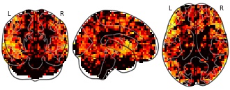
Collection description

Subject species

homo sapiens

Map type

Other

The purpose of the Colorado All-Lands Quantitative Wildfire Risk Assessment (COAL) for the USFS Rocky Mountain Region (R2) is to provide foundational information about wildfire hazard and risk to highly valued resources and assets across all land ownerships in the state of Colorado. Such information supports fuel management planning decisions, as well as revisions to land and resource management plans. A wildfire risk assessment is a quantitative analysis of assets and resources and how they would be potentially impacted by wildfire. The COAL analysis considers several different components, each resolved spatially across the project area, including:likelihood of a fire burning;the intensity of a fire if one should occur;the exposure of assets and resources based on their locations;the susceptibility of those assets and resources to wildfire.This data is part of the COAL 'fuelscape', which is a data stack or collection of raster files that describe the fuel and physical environment for a given spatial extent used in fire behavior modeling. The fuelscape is also referred to as the Farsite/FlamMap data sandwich, Farsite/FlamMap landscape files, (LCP) and similar notations.Starting with the baseline customized COAL canopy base height dataset developed following calibration workshops and actual disturbances through the 2020 field season, treated canopy base height values in this dataset were altered based on their corresponding Existing Vegetation Type following pre-identified map logic established by Landfire Rulesets Database. Each Existing Vegetation Type (EVT) corresponded to hypothetical yet theoretically appropriate generic treatment type (prescribed fire, mechanical-only, mechanical with fire, etc.). Each treatment type corresponded to predetermined set of values that raised canopy base height, specified in the pre-identified map logic. The values in the hypothetical treated canopy base height were thus modified. Treatment type and severity are sensitive to existing vegetation type and canopy cover percent; hence some areas were designated as untreatable if they did not meet the EVT and Canopy Cover map logic.The treated canopy base height is designed to identify at a coarse scale areas of the landscape where fuel treatments may have benefit based on Existing Vegetation Type and canopy cover, corresponding with pre-determined map logic. Additional analysis is required at finer scales and with other relevant datasets to identify operational and realistic opportunities to treat or affect change. The hypothetical treated canopy base height dataset was utilized to update the fire distribution (FDIST) datasets for model purposes to simulate a hypothetical disturbance as a treatment.For more information regarding quantitative wildfire risk assessment, please refer to GTR-315: https://www.fs.usda.gov/rm/pubs/rmrs_gtr315.pdf.For information about the COAL QWRA, please refer to the COAL report: https://pyrologix.com/download.For details about Landfire treated map logic, refer to Landfire Rulesets Database: https://www.landfire.gov/fuel_rulesets_db.php.This dataset was developed for the Rocky Mountain Region of the U.S. Forest Service (USFS) by Pyrologix LLC.