- a
Mapping Clusters: Hot Spot and Cluster and Outlier Analysis
- hub.arcgis.com
Updated Nov 8, 2019 Share
Share Facebook
 Twitter
 EmailClick to copy linkLink copiedCiteState of Delaware (2019). Mapping Clusters: Hot Spot and Cluster and Outlier Analysis [Dataset]. https://hub.arcgis.com/documents/delaware::mapping-clusters-hot-spot-and-cluster-and-outlier-analysis/aboutDataset updatedNov 8, 2019Dataset authored and provided byState of DelawareDescription
This course will introduce you to two of these tools: the Hot Spot Analysis (Getis-Ord Gi*) tool and the Cluster and Outlier Analysis (Anselin Local Moran's I) tool. These tools provide you with more control over your analysis. You can also use these tools to refine your analysis so that it better meets your needs.GoalsAnalyze data using the Hot Spot Analysis (Getis-Ord Gi*) tool.Analyze data using the Cluster and Outlier Analysis (Anselin Local Moran's I) tool.
- f
Sorting data.
- figshare.com
- plos.figshare.com
txtUpdated Nov 30, 2023+ more versionsShareFacebookTwitterEmailClick to copy linkLink copiedCiteWaad R. Alolayan; Jana M. Rieger; Minn N. Yoon (2023). Sorting data. [Dataset]. http://doi.org/10.1371/journal.pone.0294712.s010txtAvailable download formatsUnique identifierhttps://doi.org/10.1371/journal.pone.0294712.s010Dataset updatedNov 30, 2023Dataset provided byPLOS ONEAuthorsWaad R. Alolayan; Jana M. Rieger; Minn N. YoonLicenseAttribution 4.0 (CC BY 4.0)https://creativecommons.org/licenses/by/4.0/
License information was derived automaticallyDescriptionWith the increasing focus on patient-centred care, this study sought to understand priorities considered by patients and healthcare providers from their experience with head and neck cancer treatment, and to compare how patients’ priorities compare to healthcare providers’ priorities. Group concept mapping was used to actively identify priorities from participants (patients and healthcare providers) in two phases. In phase one, participants brainstormed statements reflecting considerations related to their experience with head and neck cancer treatment. In phase two, statements were sorted based on their similarity in theme and rated in terms of their priority. Multidimensional scaling and cluster analysis were performed to produce multidimensional maps to visualize the findings. Two-hundred fifty statements were generated by participants in the brainstorming phase, finalized to 94 statements that were included in phase two. From the sorting activity, a two-dimensional map with stress value of 0.2213 was generated, and eight clusters were created to encompass all statements. Timely care, education, and person-centred care were the highest rated priorities for patients and healthcare providers. Overall, there was a strong correlation between patient and healthcare providers’ ratings (r = 0.80). Our findings support the complexity of the treatment planning process in head and neck cancer, evident by the complex maps and highly interconnected statements related to the experience of treatment. Implications for improving the quality of care delivered and care experience of head and cancer are discussed.
Canadian Cluster Map Portal Data
- open.canada.ca
csvUpdated Feb 21, 2022+ more versionsShareFacebookTwitterEmailClick to copy linkLink copiedCiteInnovation, Science and Economic Development Canada (2022). Canadian Cluster Map Portal Data [Dataset]. https://open.canada.ca/data/en/dataset/83c19800-74a9-4da5-8d67-d2e0611e167fcsvAvailable download formatsDataset updatedFeb 21, 2022LicenseOpen Government Licence - Canada 2.0https://open.canada.ca/en/open-government-licence-canada
License information was derived automaticallyTime period coveredJan 1, 2006 - Dec 31, 2017Area coveredCanadaDescriptionThe datasets provided encompass all the statistics found on the Canadian Cluster Map Portal. Moreover, additional information such as cluster-concordance and cluster descriptions are provided to allow for accurate analysis of the data.
- a
Wards BioGeoPhysical Clusters
- hub.arcgis.com
Updated Oct 27, 2022+ more versionsShareFacebookTwitterEmailClick to copy linkLink copiedCitegISU (2022). Wards BioGeoPhysical Clusters [Dataset]. https://hub.arcgis.com/maps/4b455b84a9cd496c8cc0308226bab0d5_0/exploreDataset updatedOct 27, 2022Dataset authored and provided bygISUArea coveredDescriptionSee Publication: https://doi.org/10.1002/ecs2.4242 Policy interest in socio-ecological systems has driven attempts to define and map socio-ecological zones (SEZs), that is, spatial regions, distinguishable by their conjoined social and bio-geo-physical characteristics. The state of Idaho, USA, has a strong need for SEZ designations because of potential conflicts between rapidly increasing and impactful human populations, and proximal natural ecosystems. Our Idaho SEZs address analytical shortcomings in previously published SEZs by: (1) considering potential biases of clustering methods, (2) cross-validating SEZ classifications, (3) measuring the relative importance of bio-geo-physical and social system predictors, and (4) considering spatial autocorrelation. We obtained authoritative bio-geo-physical and social system datasets for Idaho, aggregated into 5-km grids = 25 km2, and decomposed these using principal components analyses (PCAs). PCA scores were classified using two clustering techniques commonly used in SEZ mapping: hierarchical clustering with Ward's linkage, and k-means analysis. Classification evaluators indicated that eight- and five-cluster solutions were optimal for the bio-geo-physical and social datasets for Ward's linkage, resulting in 31 SEZ composite types, and six- and five-cluster solutions were optimal for k-means analysis, resulting in 24 SEZ composite types. Ward's and k-means solutions were similar for bio-geo-physical and social classifications with similar numbers of clusters. Further, both classifiers identified the same dominant SEZ composites. For rarer SEZs, however, classification methods strongly affected SEZ classifications, potentially altering land management perspectives. Our SEZs identify several critical regions of social–ecological overlap. These include suburban interface types and a high desert transition zone. Based on multinomial generalized linear models, bio-geo-physical information explained more variation in SEZs than social system data, after controlling for spatial autocorrelation, under both Ward's and k-means approaches. Agreement (cross-validation) levels were high for multinomial models with bio-geo-physical and social predictors for both Ward's and k-means SEZs. A consideration of historical drivers, including indigenous social systems, and current trajectories of land and resource management in Idaho, indicates a strong need for rigorous SEZ designations to guide development and conservation in the region. Our analytical framework can be broadly applied in SES research and applied in other regions, when categorical responses—including cluster designations—have a spatial component.
- N
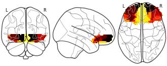
Connectivity-Based Parcellation of the Human Orbitofrontal Cortex: K=7...
- neurovault.org
niftiUpdated Nov 18, 2024+ more versionsShareFacebookTwitterEmailClick to copy linkLink copiedCite(2024). Connectivity-Based Parcellation of the Human Orbitofrontal Cortex: K=7 cluster map [Dataset]. http://identifiers.org/neurovault.image:887628niftiAvailable download formatsUnique identifierhttps://identifiers.org/neurovault.image:887628Dataset updatedNov 18, 2024LicenseCC0 1.0 Universal Public Domain Dedicationhttps://creativecommons.org/publicdomain/zero/1.0/
License information was derived automaticallyDescriptionK=7 cluster map based on N=13 participants.
Collection description
K-means cluster maps of orbitofrontal cortex with K=2, 3, 4, 5, 6, and 7 clusters based on resting-state fMRI data.
Subject species
homo sapiens
Modality
fMRI-BOLD
Analysis level
group
Cognitive paradigm (task)
rest eyes open
Map type
R
- a
Kmeans Socio Economic Clusters
- hub.arcgis.com
Updated Feb 15, 2023ShareFacebookTwitterEmailClick to copy linkLink copiedCitegISU (2023). Kmeans Socio Economic Clusters [Dataset]. https://hub.arcgis.com/maps/ISU::kmeans-socio-economic-clustersDataset updatedFeb 15, 2023Dataset authored and provided bygISUArea coveredDescriptionSee Publication: https://doi.org/10.1002/ecs2.4242 Policy interest in socio-ecological systems has driven attempts to define and map socio-ecological zones (SEZs), that is, spatial regions, distinguishable by their conjoined social and bio-geo-physical characteristics. The state of Idaho, USA, has a strong need for SEZ designations because of potential conflicts between rapidly increasing and impactful human populations, and proximal natural ecosystems. Our Idaho SEZs address analytical shortcomings in previously published SEZs by: (1) considering potential biases of clustering methods, (2) cross-validating SEZ classifications, (3) measuring the relative importance of bio-geo-physical and social system predictors, and (4) considering spatial autocorrelation. We obtained authoritative bio-geo-physical and social system datasets for Idaho, aggregated into 5-km grids = 25 km2, and decomposed these using principal components analyses (PCAs). PCA scores were classified using two clustering techniques commonly used in SEZ mapping: hierarchical clustering with Ward's linkage, and k-means analysis. Classification evaluators indicated that eight- and five-cluster solutions were optimal for the bio-geo-physical and social datasets for Ward's linkage, resulting in 31 SEZ composite types, and six- and five-cluster solutions were optimal for k-means analysis, resulting in 24 SEZ composite types. Ward's and k-means solutions were similar for bio-geo-physical and social classifications with similar numbers of clusters. Further, both classifiers identified the same dominant SEZ composites. For rarer SEZs, however, classification methods strongly affected SEZ classifications, potentially altering land management perspectives. Our SEZs identify several critical regions of social–ecological overlap. These include suburban interface types and a high desert transition zone. Based on multinomial generalized linear models, bio-geo-physical information explained more variation in SEZs than social system data, after controlling for spatial autocorrelation, under both Ward's and k-means approaches. Agreement (cross-validation) levels were high for multinomial models with bio-geo-physical and social predictors for both Ward's and k-means SEZs. A consideration of historical drivers, including indigenous social systems, and current trajectories of land and resource management in Idaho, indicates a strong need for rigorous SEZ designations to guide development and conservation in the region. Our analytical framework can be broadly applied in SES research and applied in other regions, when categorical responses—including cluster designations—have a spatial component.
- f
Clusters indicated as mapping priorities with their constituent diseases...
- datasetcatalog.nlm.nih.gov
- plos.figshare.com
Updated Jun 10, 2015ShareFacebookTwitterEmailClick to copy linkLink copiedCiteDowell, Scott F.; Krause, L. Kendall; Kimball, Ann M.; Battle, Katherine E.; Howes, Rosalind E.; Kyu, Hmwe H.; Wiebe, Antoinette; Gething, Peter W.; Farag, Tamer H.; Murray, Christopher J. L.; Pigott, David M.; Hay, Simon I.; Brooker, Simon J.; Smith, Craig H.; Vos, Theo; Golding, Nick; Garcia, Andres J.; Moyes, Catherine L. (2015). Clusters indicated as mapping priorities with their constituent diseases recommended for distribution modelling and current global mapping projects identified. [Dataset]. https://datasetcatalog.nlm.nih.gov/dataset?q=0001872787Dataset updatedJun 10, 2015AuthorsDowell, Scott F.; Krause, L. Kendall; Kimball, Ann M.; Battle, Katherine E.; Howes, Rosalind E.; Kyu, Hmwe H.; Wiebe, Antoinette; Gething, Peter W.; Farag, Tamer H.; Murray, Christopher J. L.; Pigott, David M.; Hay, Simon I.; Brooker, Simon J.; Smith, Craig H.; Vos, Theo; Golding, Nick; Garcia, Andres J.; Moyes, Catherine L.Description- Indicates default null value.MAP—Malaria Atlas Project; WHO—World Health Organization; GBD—Global Burden of Disease; GAHI—Global Atlas of Helminth Infections; SEEG—Spatial Ecology and Epidemiology Group; APOC—African Programme for Onchocerciasis Control; GAT—Global Atlas of TrachomaClusters indicated as mapping priorities with their constituent diseases recommended for distribution modelling and current global mapping projects identified.
- f
KEGG biochemical mapping for D. destructor clusters.
- datasetcatalog.nlm.nih.gov
Updated Jul 29, 2013ShareFacebookTwitterEmailClick to copy linkLink copiedCitePeng, Huan; Gao, Bing-li; Peng, De-liang; Huang, Wen-kun; Long, Hai-bo; He, Xu-feng; Kong, Ling-an; Yu, Qing (2013). KEGG biochemical mapping for D. destructor clusters. [Dataset]. https://datasetcatalog.nlm.nih.gov/dataset?q=0001712629Dataset updatedJul 29, 2013AuthorsPeng, Huan; Gao, Bing-li; Peng, De-liang; Huang, Wen-kun; Long, Hai-bo; He, Xu-feng; Kong, Ling-an; Yu, QingDescriptionKEGG biochemical mapping for D. destructor clusters.
- f
World Clusters map
- data.apps.fao.org
Updated Mar 1, 2024ShareFacebookTwitterEmailClick to copy linkLink copiedCite(2024). World Clusters map [Dataset]. https://data.apps.fao.org/map/catalog/srv/resources/registries/vocabularies//concepts/Tag_landDataset updatedMar 1, 2024Area coveredWorldDescriptionWorld cluster map of the world based on a Coastal zone (LOICZ) database received in 1995 from the Netherlands Institute for Sea Research (NIOZ).
- S
Detailed Connectomic Cluster Resource for White Matter Mapping From...
- scidb.cn
Updated Aug 22, 2025ShareFacebookTwitterEmailClick to copy linkLink copiedCiteYifei He; Wu Ye (2025). Detailed Connectomic Cluster Resource for White Matter Mapping From Ultra-High-Field Diffusion MRI [Dataset]. http://doi.org/10.57760/sciencedb.28989CroissantCroissant is a format for machine-learning datasets. Learn more about this at mlcommons.org/croissant.Unique identifierhttps://doi.org/10.57760/sciencedb.28989Dataset updatedAug 22, 2025Dataset provided byScience Data BankAuthorsYifei He; Wu YeLicenseAttribution 4.0 (CC BY 4.0)https://creativecommons.org/licenses/by/4.0/
License information was derived automaticallyDescriptionWe develop a data-driven fiber-cluster atlas utilizing ultra-high-field 7T structural and diffusion MRI data from 171 Human Connectome Project (HCP) participants. We cluster streamlines connecting seven cortical networks and nine subcortical regions using cosine k-means clustering alongside two-level consensus filtering. The resulting atlas comprises 33,256 clusters for a seven-network scheme and 65,184 clusters for a seventeen-network scheme, encompassing both deep and superficial white matter.
- Z
Data from: Copernicus Global Land Service: Global biome cluster layer for...
- data.niaid.nih.gov
- zenodo.org
Updated Jan 14, 2022ShareFacebookTwitterEmailClick to copy linkLink copiedCiteMarcel Buchhorn (2022). Copernicus Global Land Service: Global biome cluster layer for the 100m global land cover processing line [Dataset]. https://data.niaid.nih.gov/resources?id=zenodo_5848609Dataset updatedJan 14, 2022Dataset provided byVITO NVAuthorsMarcel BuchhornLicenseAttribution 4.0 (CC BY 4.0)https://creativecommons.org/licenses/by/4.0/
License information was derived automaticallyDescriptionA map of 73 global biome clusters, geographic areas that were grouped to optimize the global 100m land cover processing.
In order to group Earth Observation data for faster processing or adaptation of algorithms to specific regions, the 100m global land cover (CGLS-LC100) algorithm uses a Global Biome Cluster layer. The term biome cluster hereby refers to a geographic area which has similar bio-geophysical parameters and, therefore, can be grouped for processing. In other words, the biome cluster layer can be seen as an ecological regionalisation which outlines areas of similar environmental conditions, ecological processes, and biotic communities (Coops et al., 2018). There are already several global regionalisation layers existing, e.g. Ecoregions 2017 global dataset (Dinerstein et al., 2017), Geiger-Koeppen global ecozones after Olofsson update (Olofsson et al., 2012), Global ecological zones for FAO forest reporting with update 2010 (FAO, 2012). But several tests in the CGLS-LC100 workflow have shown that the existing layers did not provide the required global and continental classification accuracy. These findings go along with Coops et al. (2018) who stated that "Most regionalisations are made based on subjective criteria, and cannot be readily revised, leading to outstanding questions with respect to how to optimally develop and define them."
Therefore, we decided to develop a customized ecological regionalisation layer which performs best with the given PROBA-V remote sensing data and the specifications of the CGLS-LC100 product. It groups spectral similar areas and helps to optimize the later classification/regression to regional patterns. Input into the layer creation were well-known existing datasets which were combined, re-grouped and advanced based on prior CGLS-LC100 classification results and local mapping knowledge of the workflow developer. To ensure that this layer is clearly separable from other existing regionalisations and not mistakenly interpreted as an eco-region layer, we decide to call it biome clusters layer.
The following steps outline the global biome clusters layer generation:
Spatial union of Ecoregions 2017 dataset (Dinerstein et al., 2017), Geiger-Koeppen dataset (Olofsson et al., 2012) and Global FAO eco-regions datasets (FAO, 2012);
Regrouping and dissolving by using experience from first global CGLS-LC100 mapping results and subjective mapping experience of the developer;
Refinement of the biome clusters in the High North latitudes via incorporation of a Global tree-line layer (Alaska Geobotany Center, 2003);
Manual improvement of borders between biome clusters to reduce classification artefacts by using a DEM and mapping experience from previous projects and continental test runs;
Usage of a global land/sea mask, the Sentinel-2 tiling grid and PROBA-V imaging extent to extend the borders of the biome clusters into the sea to make sure that also small islands on the coastline are correctly processed.
When developing a regionalisation, the definition of the clusters and the boundaries that delineate them in time and space is the key challenge. Overall, the map distinguishes 73 global biome clusters.
- d
Linkage disequilibrium clustering-based approach for association mapping...
- datadryad.org
- data.niaid.nih.gov
zipUpdated Apr 12, 2018ShareFacebookTwitterEmailClick to copy linkLink copiedCiteZitong Li; Petri Kemppainen; Pasi Rastas; Juha Merilä (2018). Linkage disequilibrium clustering-based approach for association mapping with tightly linked genome-wide data [Dataset]. http://doi.org/10.5061/dryad.16g72gkzipAvailable download formatsUnique identifierhttps://doi.org/10.5061/dryad.16g72gkDataset updatedApr 12, 2018Dataset provided byDryadAuthorsZitong Li; Petri Kemppainen; Pasi Rastas; Juha MeriläTime period coveredApr 5, 2018DescriptionR script and code for cluster-based association and QTL mappingR script and example data for cluster-based association and QTL mapping.zip
- m
2019-2021 HSIP Cluster
- gis.data.mass.gov
- geo-massdot.opendata.arcgis.com
- +3more
Updated Jul 2, 2024+ more versionsShareFacebookTwitterEmailClick to copy linkLink copiedCiteMassachusetts geoDOT (2024). 2019-2021 HSIP Cluster [Dataset]. https://gis.data.mass.gov/datasets/MassDOT::2019-2021-hsip-cluster-Dataset updatedJul 2, 2024Dataset authored and provided byMassachusetts geoDOTArea coveredDescriptionThe top locations where reported collisions occurred at intersections have been identified. The crash cluster analysis methodology for the top intersection clusters uses a fixed meter search distance of 25 meters (82 ft.) to merge crash clusters together. This analysis was based on crashes where a police officer specified one of the following junction types: Four way intersection, T-intersection, Y-intersection, five point or more. Furthermore, the methodology uses the Equivalent Property Damage Only (EPDO) weighting to rank the clusters. EPDO is based any type of injury crash (including fatal, incapacitating, non-incapacitating and possible) having a weighting of 21 compared to a property damage only crash (which has weighting of 1). The clustering analysis used crashes from the three year period from 2019-2021. The area encompassing the crash cluster may cover a larger area than just the intersection so it is critical to view these spatially.
Clusters of interactions common between the Parkinson's disease map and the...
- data-staging.niaid.nih.gov
- data.niaid.nih.gov
- +1more
Updated Dec 18, 2022ShareFacebookTwitterEmailClick to copy linkLink copiedCiteMarek Ostaszewski (2022). Clusters of interactions common between the Parkinson's disease map and the Ageing map [Dataset]. https://data-staging.niaid.nih.gov/resources?id=zenodo_7448588Dataset updatedDec 18, 2022Dataset provided byLuxembourg Centre for Systems BiomedicineAuthorsMarek OstaszewskiLicenseAttribution 4.0 (CC BY 4.0)https://creativecommons.org/licenses/by/4.0/
License information was derived automaticallyDescriptionThis set of files was generated using the script demonstrating the use of MINERVA Net repository.
The script is available under:
https://gitlab.lcsb.uni.lu/minerva/api-scripts/-/blob/master/R/API-minervanet.R
The diagrams should be opened with the CellDesigner software (https://www.celldesigner.org/).
- r
Data from: Discovering biogeographic and ecological clusters with a graph...
- researchdata.edu.au
- figshare.mq.edu.au
- +3more
Updated Jun 12, 2022+ more versionsShareFacebookTwitterEmailClick to copy linkLink copiedCiteJohn Alroy (2022). Data from: Discovering biogeographic and ecological clusters with a graph theoretic spin on factor analysis [Dataset]. http://doi.org/10.5061/DRYAD.R48D279Unique identifierhttps://doi.org/10.5061/DRYAD.R48D279Dataset updatedJun 12, 2022Dataset provided byMacquarie UniversityAuthorsJohn AlroyDescriptionFactor analysis (FA) has the advantage of highlighting each semi-distinct cluster of samples in a data set with one axis at a time, as opposed to simply arranging samples across axes to represent gradients. However, in the case of presence-absence data it is confounded by absences when gradients are long. No statistical model can cope with this problem because the raw data simply do not present underlying information about the length of such gradients. Here I propose a simple way to tease out this information. It is a simple emendation of FA called stepping down, which involves giving an absence a negative value when the missing species nowhere co-occurs with the species found in the relevant sample. Specifically, a binary co-occurrence graph is created, and the magnitude of negative values is made a function of how far the graph must be traversed in order to link the missing species with each species that is present. Simulations show that standard FA yields inferior results to FA based on stepped-down matrices in terms of mapping clusters into axes one-by-one. Standard FA is also uninformative when applied to a global bat inventory data set. Step-down FA (SDFA) easily flags the main biogeographic groupings. Methods like correspondence analysis, non-metric multidimensional scaling, and Bayesian latent variable modelling are not commensurate with SDFA because they do not seek to find a one-to-one mapping of axes and clusters. Stepping down seems promising as a means of illustrating clusters of samples, especially when there are subtle or complex discontinuities in gradients.
Usage Notes
bat referencesA list of references to publications yielding site-specific inventory data for bats from around the world. Raw data are also reposited in the Ecological Register.bat_references.txtbat registerSite-specific inventory data for bats from around the world. Each line includes a count of the individuals belonging to a species found at a site. Raw data are also reposited in the Ecological Register.bat_register.txt
- m
Educational Attainment in North Carolina Public Schools: Use of statistical...
- data.mendeley.com
Updated Nov 14, 2018ShareFacebookTwitterEmailClick to copy linkLink copiedCiteScott Herford (2018). Educational Attainment in North Carolina Public Schools: Use of statistical modeling, data mining techniques, and machine learning algorithms to explore 2014-2017 North Carolina Public School datasets. [Dataset]. http://doi.org/10.17632/6cm9wyd5g5.1Unique identifierhttps://doi.org/10.17632/6cm9wyd5g5.1Dataset updatedNov 14, 2018AuthorsScott HerfordLicenseAttribution 4.0 (CC BY 4.0)https://creativecommons.org/licenses/by/4.0/
License information was derived automaticallyDescriptionThe purpose of data mining analysis is always to find patterns of the data using certain kind of techiques such as classification or regression. It is not always feasible to apply classification algorithms directly to dataset. Before doing any work on the data, the data has to be pre-processed and this process normally involves feature selection and dimensionality reduction. We tried to use clustering as a way to reduce the dimension of the data and create new features. Based on our project, after using clustering prior to classification, the performance has not improved much. The reason why it has not improved could be the features we selected to perform clustering are not well suited for it. Because of the nature of the data, classification tasks are going to provide more information to work with in terms of improving knowledge and overall performance metrics. From the dimensionality reduction perspective: It is different from Principle Component Analysis which guarantees finding the best linear transformation that reduces the number of dimensions with a minimum loss of information. Using clusters as a technique of reducing the data dimension will lose a lot of information since clustering techniques are based a metric of 'distance'. At high dimensions euclidean distance loses pretty much all meaning. Therefore using clustering as a "Reducing" dimensionality by mapping data points to cluster numbers is not always good since you may lose almost all the information. From the creating new features perspective: Clustering analysis creates labels based on the patterns of the data, it brings uncertainties into the data. By using clustering prior to classification, the decision on the number of clusters will highly affect the performance of the clustering, then affect the performance of classification. If the part of features we use clustering techniques on is very suited for it, it might increase the overall performance on classification. For example, if the features we use k-means on are numerical and the dimension is small, the overall classification performance may be better. We did not lock in the clustering outputs using a random_state in the effort to see if they were stable. Our assumption was that if the results vary highly from run to run which they definitely did, maybe the data just does not cluster well with the methods selected at all. Basically, the ramification we saw was that our results are not much better than random when applying clustering to the data preprocessing. Finally, it is important to ensure a feedback loop is in place to continuously collect the same data in the same format from which the models were created. This feedback loop can be used to measure the model real world effectiveness and also to continue to revise the models from time to time as things change.
Mapping color space to 100 color names
- kaggle.com
Updated Jun 24, 2022ShareFacebookTwitterEmailClick to copy linkLink copiedCiteGoldNuss (2022). Mapping color space to 100 color names [Dataset]. https://www.kaggle.com/datasets/danela/mapping-color-space-to-100-color-namesCroissantCroissant is a format for machine-learning datasets. Learn more about this at mlcommons.org/croissant.Dataset updatedJun 24, 2022Dataset provided byKaggleAuthorsGoldNussDescriptionDataset to segment RGB colour space into 100 colour names. Each point in colour space can be assigned to a colour name by finding the nearest neighbour.
Data contains 100 colour names which correspond to well-distributed coordinates in RGB-colour space. The data were obtained by clustering more than 1000 colours from joined data sets from xkcd (https://xkcd.com/color/rgb/, https://xkcd.com/color/satfaces.txt) and the webcolors package (https://github.com/ubernostrum/webcolors) to 100 clusters using KMeans.
- d
Datasets for Computational Methods and GIS Applications in Social Science
- search.dataone.org
Updated Oct 29, 2025ShareFacebookTwitterEmailClick to copy linkLink copiedCiteFahui Wang; Lingbo Liu (2025). Datasets for Computational Methods and GIS Applications in Social Science [Dataset]. http://doi.org/10.7910/DVN/4CM7V4Unique identifierhttps://doi.org/10.7910/DVN/4CM7V4Dataset updatedOct 29, 2025Dataset provided byHarvard DataverseAuthorsFahui Wang; Lingbo LiuDescriptionDataset for the textbook Computational Methods and GIS Applications in Social Science (3rd Edition), 2023 Fahui Wang, Lingbo Liu Main Book Citation: Wang, F., & Liu, L. (2023). Computational Methods and GIS Applications in Social Science (3rd ed.). CRC Press. https://doi.org/10.1201/9781003292302 KNIME Lab Manual Citation: Liu, L., & Wang, F. (2023). Computational Methods and GIS Applications in Social Science - Lab Manual. CRC Press. https://doi.org/10.1201/9781003304357 KNIME Hub Dataset and Workflow for Computational Methods and GIS Applications in Social Science-Lab Manual Update Log If Python package not found in Package Management, use ArcGIS Pro's Python Command Prompt to install them, e.g., conda install -c conda-forge python-igraph leidenalg NetworkCommDetPro in CMGIS-V3-Tools was updated on July 10,2024 Add spatial adjacency table into Florida on June 29,2024 The dataset and tool for ABM Crime Simulation were updated on August 3, 2023, The toolkits in CMGIS-V3-Tools was updated on August 3rd,2023. Report Issues on GitHub https://github.com/UrbanGISer/Computational-Methods-and-GIS-Applications-in-Social-Science Following the website of Fahui Wang : http://faculty.lsu.edu/fahui Contents Chapter 1. Getting Started with ArcGIS: Data Management and Basic Spatial Analysis Tools Case Study 1: Mapping and Analyzing Population Density Pattern in Baton Rouge, Louisiana Chapter 2. Measuring Distance and Travel Time and Analyzing Distance Decay Behavior Case Study 2A: Estimating Drive Time and Transit Time in Baton Rouge, Louisiana Case Study 2B: Analyzing Distance Decay Behavior for Hospitalization in Florida Chapter 3. Spatial Smoothing and Spatial Interpolation Case Study 3A: Mapping Place Names in Guangxi, China Case Study 3B: Area-Based Interpolations of Population in Baton Rouge, Louisiana Case Study 3C: Detecting Spatiotemporal Crime Hotspots in Baton Rouge, Louisiana Chapter 4. Delineating Functional Regions and Applications in Health Geography Case Study 4A: Defining Service Areas of Acute Hospitals in Baton Rouge, Louisiana Case Study 4B: Automated Delineation of Hospital Service Areas in Florida Chapter 5. GIS-Based Measures of Spatial Accessibility and Application in Examining Healthcare Disparity Case Study 5: Measuring Accessibility of Primary Care Physicians in Baton Rouge Chapter 6. Function Fittings by Regressions and Application in Analyzing Urban Density Patterns Case Study 6: Analyzing Population Density Patterns in Chicago Urban Area >Chapter 7. Principal Components, Factor and Cluster Analyses and Application in Social Area Analysis Case Study 7: Social Area Analysis in Beijing Chapter 8. Spatial Statistics and Applications in Cultural and Crime Geography Case Study 8A: Spatial Distribution and Clusters of Place Names in Yunnan, China Case Study 8B: Detecting Colocation Between Crime Incidents and Facilities Case Study 8C: Spatial Cluster and Regression Analyses of Homicide Patterns in Chicago Chapter 9. Regionalization Methods and Application in Analysis of Cancer Data Case Study 9: Constructing Geographical Areas for Mapping Cancer Rates in Louisiana Chapter 10. System of Linear Equations and Application of Garin-Lowry in Simulating Urban Population and Employment Patterns Case Study 10: Simulating Population and Service Employment Distributions in a Hypothetical City Chapter 11. Linear and Quadratic Programming and Applications in Examining Wasteful Commuting and Allocating Healthcare Providers Case Study 11A: Measuring Wasteful Commuting in Columbus, Ohio Case Study 11B: Location-Allocation Analysis of Hospitals in Rural China Chapter 12. Monte Carlo Method and Applications in Urban Population and Traffic Simulations Case Study 12A. Examining Zonal Effect on Urban Population Density Functions in Chicago by Monte Carlo Simulation Case Study 12B: Monte Carlo-Based Traffic Simulation in Baton Rouge, Louisiana Chapter 13. Agent-Based Model and Application in Crime Simulation Case Study 13: Agent-Based Crime Simulation in Baton Rouge, Louisiana Chapter 14. Spatiotemporal Big Data Analytics and Application in Urban Studies Case Study 14A: Exploring Taxi Trajectory in ArcGIS Case Study 14B: Identifying High Traffic Corridors and Destinations in Shanghai Dataset File Structure 1 BatonRouge Census.gdb BR.gdb 2A BatonRouge BR_Road.gdb Hosp_Address.csv TransitNetworkTemplate.xml BR_GTFS Google API Pro.tbx 2B Florida FL_HSA.gdb R_ArcGIS_Tools.tbx (RegressionR) 3A China_GX GX.gdb 3B BatonRouge BR.gdb 3C BatonRouge BRcrime R_ArcGIS_Tools.tbx (STKDE) 4A BatonRouge BRRoad.gdb 4B Florida FL_HSA.gdb HSA Delineation Pro.tbx Huff Model Pro.tbx FLplgnAdjAppend.csv 5 BRMSA BRMSA.gdb Accessibility Pro.tbx 6 Chicago ChiUrArea.gdb R_ArcGIS_Tools.tbx (RegressionR) 7 Beijing BJSA.gdb bjattr.csv R_ArcGIS_Tools.tbx (PCAandFA, BasicClustering) 8A Yunnan YN.gdb R_ArcGIS_Tools.tbx (SaTScanR) 8B Jiangsu JS.gdb 8C Chicago ChiCity.gdb cityattr.csv ...
- d
Data from: Database for the Geologic Map of Three Sisters Volcanic Cluster,...
- catalog.data.gov
- data.usgs.gov
- +1more
Updated Nov 21, 2025+ more versionsShareFacebookTwitterEmailClick to copy linkLink copiedCiteU.S. Geological Survey (2025). Database for the Geologic Map of Three Sisters Volcanic Cluster, Cascade Range, Oregon [Dataset]. https://catalog.data.gov/dataset/database-for-the-geologic-map-of-three-sisters-volcanic-cluster-cascade-range-oregonDataset updatedNov 21, 2025Area coveredCascade Range, Three Sisters, OregonDescriptionA database of geologic map of Three Sisters Volcanic Cluster as described in the original abstract: The geologic map represents part of a late Quaternary volcanic field within which scores of eruptions have taken place over the last 50,000 years, some as recently as ~1,500 years ago. No rocks of early Pleistocene (or greater) age crop out within the map area, although volcanic and derivative sedimentary rocks of Miocene and Pliocene age are widespread to the east and west and are certainly buried beneath the younger volcanic field. Of the 145 volcanic map units described herein, only 22 are certainly older than late Pleistocene (>126 ka), and 12 are postglacial (<15 ka). The oldest unit identified yields an age of 532+/-7 ka, and the second oldest, 374+/-6 ka. Compositionally, 10 percent of the units are true basalt; 36 percent, basaltic andesite; 20 percent, andesite; 21.5 percent, dacite; and only 12.5 percent, rhyodacite or rhyolite. Most of the 145 volcanic map units described herein are newly defined, although equivalents of several were described by Taylor, 1978, 1987; Scott, 1987; and Scott and Gardner, 1992. Each is an eruptive unit derived from a single vent or fissure. Some are simple flow units, but many are shields, cones, or stacks of several lava flows that have chemical and mineralogical coherence. Each unit was delineated by field mapping on foot and its integrity confirmed, challenged, or revised by chemical and microscopic work in the laboratory. Definition of a few units required iterative acquisition of field and lab data over a period of years, providing a firm basis for subdividing, lumping, or correlating slightly heterogeneous sequences of lavas. Most units have narrow compositional ranges, but some show zoning or heterogeneity spanning ranges of a few percent SiO2.
- d
Neighborhood Clusters
- catalog.data.gov
- opendata.dc.gov
- +1more
Updated Feb 5, 2025+ more versionsShareFacebookTwitterEmailClick to copy linkLink copiedCiteD.C. Office of the Chief Technology Officer (2025). Neighborhood Clusters [Dataset]. https://catalog.data.gov/dataset/neighborhood-clustersDataset updatedFeb 5, 2025Dataset provided byD.C. Office of the Chief Technology OfficerDescriptionThis data set describes Neighborhood Clusters that have been used for community planning and related purposes in the District of Columbia for many years. It does not represent boundaries of District of Columbia neighborhoods. Cluster boundaries were established in the early 2000s based on the professional judgment of the staff of the Office of Planning as reasonably descriptive units of the City for planning purposes. Once created, these boundaries have been maintained unchanged to facilitate comparisons over time, and have been used by many city agencies and outside analysts for this purpose. (The exception is that 7 “additional” areas were added to fill the gaps in the original dataset, which omitted areas without significant neighborhood character such as Rock Creek Park, the National Mall, and the Naval Observatory.) The District of Columbia does not have official neighborhood boundaries. The Office of Planning provides a separate data layer containing Neighborhood Labels that it uses to place neighborhood names on its maps. No formal set of standards describes which neighborhoods are included in that dataset.Whereas neighborhood boundaries can be subjective and fluid over time, these Neighborhood Clusters represent a stable set of boundaries that can be used to describe conditions within the District of Columbia over time.
FacebookTwitterThis course will introduce you to two of these tools: the Hot Spot Analysis (Getis-Ord Gi*) tool and the Cluster and Outlier Analysis (Anselin Local Moran's I) tool. These tools provide you with more control over your analysis. You can also use these tools to refine your analysis so that it better meets your needs.GoalsAnalyze data using the Hot Spot Analysis (Getis-Ord Gi*) tool.Analyze data using the Cluster and Outlier Analysis (Anselin Local Moran's I) tool.