This dataset is linked to Does Zero Mean Nothing? Investigating the Attentional Mechanism of the Hidden-Zero Effect in Risky Decision-Making. In two studies, we tested the hidden-zero effect by comparing participants’ risky choices between two different conditions (i.e., presenting options with or without explicit-zero outcomes) with a full range of risky probability (from 5% to 95%). The dataset included the behavioral results (Study 1&2) and eye-movement results (Study 2) of each participants.

There is almost not a case in exploration geology, where the studied data doesn’t includes below detection limits and/or zero values, and since most of the geological data responds to lognormal distributions, these “zero data” represent a mathematical challenge for the interpretation. We need to start by recognizing that there are zero values in geology. For example the amount of quartz in a foyaite (nepheline syenite) is zero, since quartz cannot co-exists with nepheline. Another common essential zero is a North azimuth, however we can always change that zero for the value of 360°. These are known as “Essential zeros”, but what can we do with “Rounded zeros” that are the result of below the detection limit of the equipment? Amalgamation, e.g. adding Na2O and K2O, as total alkalis is a solution, but sometimes we need to differentiate between a sodic and a potassic alteration. Pre-classification into groups requires a good knowledge of the distribution of the data and the geochemical characteristics of the groups which is not always available. Considering the zero values equal to the limit of detection of the used equipment will generate spurious distributions, especially in ternary diagrams. Same situation will occur if we replace the zero values by a small amount using non-parametric or parametric techniques (imputation). The method that we are proposing takes into consideration the well known relationships between some elements. For example, in copper porphyry deposits, there is always a good direct correlation between the copper values and the molybdenum ones, but while copper will always be above the limit of detection, many of the molybdenum values will be “rounded zeros”. So, we will take the lower quartile of the real molybdenum values and establish a regression equation with copper, and then we will estimate the “rounded” zero values of molybdenum by their corresponding copper values. The method could be applied to any type of data, provided we establish first their correlation dependency. One of the main advantages of this method is that we do not obtain a fixed value for the “rounded zeros”, but one that depends on the value of the other variable.

Our objective was to model mean annual number of zero-flow days (days per year) for small streams in the Upper Colorado River Basin under historic hydrologic conditions on small, ungaged streams in the Upper Colorado River Basin. Modeling streamflows is an important tool for understanding landscape-scale drivers of flow and estimating flows where there are no gaged records. We focused our study in the Upper Colorado River Basin, a region that is not only critical for water resources but also projected to experience large future climate shifts toward a drier climate. We used a random forest modeling approach to model the relation between zero-flow days per year on gaged streams (115 gages) and environmental variables. We then projected zero-flow days per year to ungaged reaches in the Upper Colorad River Basin using environmental variables for each raster stream cell in the basin. This data layer shows modeled values for zero-flow days per year of each stream cell.

Details of Motor Vehicle Collisions in New York City provided by the Police Department (NYPD).

Means, Standard Deviations, and Zero-order Correlations (Study 8).

Mean Z-Scores (mean 0; standard deviation 1) obtained by the 15 participants in the 10 video games across the 20 training sessions.

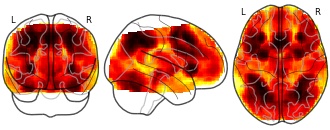
Collection description

Subject species

homo sapiens

Modality

fMRI-BOLD

Analysis level

meta-analysis

Cognitive paradigm (task)

working memory fMRI task paradigm

Map type

Other

Zero altitude, mean high tide, marine terrains and mean sea level surveys.

The eight color asteroid survey provides reflection spectra for minor planets using eight filter passbands. This dataset includes mean data averaged for each of 589 minor planets. The primary data for these minor planets, the response curves for the filters, and the values determined for standard stars, are included in other related datasets. The wavelength range covered is .33 to 1.04 micrometers.

We consider a realization of a Gaussian process with mean zero and the wave covariance function: For x, x′ ∈ [0, 10/], define the wave covariance function as √ cov(x, x′) = sin (cid:0)∥x − x′∥(cid:1).

Graph and download economic data for Weighted-Average Maturity for Zero Interval, Other Risk (Acceptable), Domestic Banks (DISCONTINUED) (EDZOXDBNQ) from Q2 1997 to Q2 2017 about zero interval, weighted-average, maturity, average, domestic, banks, depository institutions, and USA.

Asterisks indicate significant p-values (***<0.001, **<0.01, * < 0.05).

Mean consumption expenditure per household with expenditure greater than zero by COICOP consumption purpose

Average Zero-upcrossing Period for the Windsea Timeseries - North Sea - The domain is a lon/lat grid that covers the range [48.5, 57.033] in latitude and the range [-4.05, 9.25] in longitude. The latitude increment is 0.066 degrees, the longitude increment is 0.1 degrees. The spectral analysis is provided every hour. The sea surface is forced by the 1-hourly meteo forecasts provided by the ECMWF

The monthly means of NCEP/NCAR Reanalysis (R1) products, archived in ds090.0 [http://rda.ucar.edu/datasets/ds090.0/] dataset, are extracted and reorganized into subgroups in this dataset. The groupings try to combine like and/or commonly used parameter-level data together. There are also subgroups for each of the four diurnal monthly means (means of 00Z, 06Z, 12Z, and 18Z separately). The data files are in WMO GRIB format. Both the monthly means and their variances are in the same file but in different GRIB records. Examples of separating monthly means from variances are shown in this guide [http://rda.ucar.edu/datasets/ds090.2/docs/how2use_grads.txt]. All subgroups will be available on line under data [http://rda.ucar.edu/datasets/ds090.2/#access]. The ones that are not on line yet will be moved over upon request.

According to a survey conducted on zero energy houses in Japan in ***********, almost ** percent of respondents stated that the economic benefit of utility costs due to the introduction of a zero energy house ranged from around ************* to ************ Japanese yen. Overall, the average saving of utility costs due to zero energy houses amounted to ***** Japanese yen per month.

This table shows the relationship between levels of age-misreporting and migration and error in relative completeness (RC) in the simulation environment, both in the absence (a) and presence (b) of fixed effects, indicating the combination of mortality, fertility, and migration rates that define a population scenario. Error is calculated by dividing the difference between true RC and estimated RC by true RC using the optimal variant in the simulated environment for each of the three families. Stochastic age-misreporting is captured as a random draw for each individual from a normal distribution with mean zero and variance . Systematic age-misreporting is captured by the function where am is the misreported age, at is the true age, and β is drawn from a normal distribution.CI, confidence interval; RMSE, root mean squared error; VR, vital registration.

Zero altitude, mean high tide, marine terrains and mean sea level surveys.

The RSS SMAP Level 3 Sea Surface Salinity Standard Mapped Image 8-Day Running Mean V6.0 Validated Dataset produced by the Remote Sensing Systems (RSS) and sponsored by the NASA Ocean Salinity Science Team, is a validated product that provides orbital/swath data on sea surface salinity (SSS) derived from the NASA's Soil Moisture Active Passive (SMAP) mission. The SMAP satellite was launched on 31 January 2015 with a near-polar orbit at an inclination of 98 degrees and an altitude of 685 km. It has an ascending node time of 6 pm and is sun-synchronous. With its 1000km swath, SMAP achieves global coverage in approximately 3 days, but has an exact orbit repeat cycle of 8 days. Malfunction of the SMAP scatterometer on 7 July, 2015, has necessitated the use of collocated wind speed, primarily from WindSat, for the surface roughness correction required for the surface salinity retrieval.

The major changes in Version 6.0 from Version 5.0 are: (1) Removal of biases during the first few months of the SMAP mission that are related to the operation of the SMAP radar during that time. (2) Mitigation of biases that depend on the SMAP look angle. (3) Mitigation of salty biases at high Northern latitudes. (4) Revised sun-glint flag. The RSS SMAP 8-Day running mean product is based on SSS averages spanning an 8-day moving time window, it includes data for a range of parameters: derived sea surface salinity (SSS) with SSS-uncertainty, rain filtered SMAP sea surface salinity, collocated wind speed, data and ancillary reference surface salinity data from HYCOM. Each data file is available in netCDF-4 file format with about 7-day latency (after the end of the averaging period). Data begins on April 1,2015 and is ongoing. Observations are global in extent with an approximate spatial resolution of 40KM. Note that while a SSS 40KM variable is also included in the product for most open ocean applications, The standard product of the SMAP Version 6.0 release is the smoothed salinity product with a spatial resolution of approximately 70 km.

Estimate of parameters, their standard error (SE), mean ratio and p-value for different demographic and socio-economic variables obtained from Zero and One Inflated Poisson regression model.