At the end of financial year 2023, PT Mitra Adi Perkasa Tbk (MAP) reported net income of around *** trillion Indonesian rupiah. MAP is one of Indonesia's leading retail companies with a diversified portfolio ranging from sport, fashion, department stores, food & beverages to lifestyle products.

In 2023, the real median household income in the state of Alabama was 60,660 U.S. dollars. The state with the highest median household income was Massachusetts, which was 106,500 U.S. dollars in 2023. The average median household income in the United States was at 80,610 U.S. dollars.

Mapfre reported EUR192M in Net Income for its fiscal quarter ending in September of 2024. Data for Mapfre | MAP - Net Income including historical, tables and charts were last updated by Trading Economics this last August in 2025.

A dataset listing the richest zip codes in North Carolina per the most current US Census data, including information on rank and average income.

In 2000, an estimated 16 416 000 people reported employment income, an increase of more than 1.5 million from a decade earlier. During this decade, the overall average employment income of individuals rose 7.3% to $31 757. ‘Earnings’ refers to the total of wages and salaries as well as net income from self-employment.

A dataset listing the richest zip codes in Virginia per the most current US Census data, including information on rank and average income.

Unthresholded z-score map of main Net Value meta-analysis (N=15)

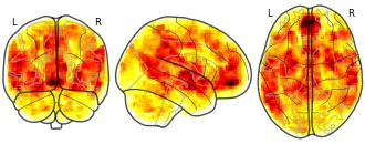
Collection description

These maps were generated by a hybrid image- and coordinate-based meta-analysis of fMRI data from effort-based decision-making studies. The goal of this meta-analysis was to determine which regions are consistently activated/deactivated in processing effort demands and net value of prospective effort-based rewards.

Subject species

homo sapiens

Modality

fMRI-BOLD

Analysis level

meta-analysis

Cognitive paradigm (task)

multi-attribute reward-guided decision task

Map type

Z

Contained within the 3rd Edition (1957) of the Atlas of Canada is a map that shows a map of six condensed maps of employment and related patterns for the leading service sectors as compiled from the 1951 Census. There are two maps referring to wholesale trade. One of them shows the distribution of the labour force engaged in wholesale trade. This is shown by a dot pattern using one dot for every 200 people of this labour force, and using proportional symbols for all places employing 2 000 or more. The other wholesale trade map shows percentage of net value of sales from wholesale trade in each census division. There are two similar maps of retail trade. One, showing the distribution of labour force, uses the same mapping procedure as that of wholesale trade. The second map shows retail trade as a percentage of net value of sales for each census division. The fifth map shows the distribution of the construction labour force, using the same mapping concepts as for the wholesale trade map. There is an associated pie chart showing the types of construction this labour force engages in. The sixth map shows the distribution of labour force in the fire, insurance and real estate industries, again using the mapping concepts used for the wholesale trade map. This map is accompanied by a pie chart showing employment in the various industries of this group (such as in banking).

This table presents income shares, thresholds, tax shares, and total counts of individual Canadian tax filers, with a focus on high income individuals (95% income threshold, 99% threshold, etc.). Income thresholds are geography-specific; for example, the number of Nova Scotians in the top 1% will be calculated as the number of taxfiling Nova Scotians whose total income exceeded the 99% income threshold of Nova Scotian tax filers. Different definitions of income are available in the table namely market, total, and after-tax income, both with and without capital gains.

Map of reported net income of tax households in 2010 by municipality. The net income declared (or tax income) of the household (www.insee.fr) consists of the resources mentioned on the income declaration, so-called declaration No. 2042. It therefore includes the accumulation of income from employment or self-employment, unemployment benefits, sickness benefits, invalidity or retirement pensions and part of income from assets. Support payments are excluded as well as exceptional income and tax-exempt wealth income (housing savings, etc.). On the other hand, income entered on declaration No 2042 and subject to a discharge levy is included (for example, income from bonds). This is the income before deductions and allowances granted by tax legislation. These incomes are net of social contributions and the generalised social contribution (CSG). The tax household (www.insee.fr) refers to all persons registered on the same tax return. There may be several tax households in a single household: for example, an unmarried couple where each completes its own tax return counts as two tax households.

WM Technology operating income from 2020 to 2025. Operating income can be defined as income after operating expenses have been deducted and before interest payments and taxes have been deducted.

Urban Displacement Project’s (UDP) Estimated Displacement Risk (EDR) model for California identifies varying levels of displacement risk for low-income renter households in all census tracts in the state from 2015 to 2019(1). The model uses machine learning to determine which variables are most strongly related to displacement at the household level and to predict tract-level displacement risk statewide while controlling for region. UDP defines displacement risk as a census tract with characteristics which, according to the model, are strongly correlated with more low-income population loss than gain. In other words, the model estimates that more low-income households are leaving these neighborhoods than moving in.This map is a conservative estimate of low-income loss and should be considered a tool to help identify housing vulnerability. Displacement may occur because of either investment, disinvestment, or disaster-driven forces. Because this risk assessment does not identify the causes of displacement, UDP does not recommend that the tool be used to assess vulnerability to investment such as new housing construction or infrastructure improvements. HCD recommends combining this map with on-the-ground accounts of displacement, as well as other related data such as overcrowding, cost burden, and income diversity to achieve a full understanding of displacement risk.If you see a tract or area that does not seem right, please fill out this form to help UDP ground-truth the method and improve their model.How should I read the displacement map layers?The AFFH Data Viewer includes three separate displacement layers that were generated by the EDR model. The “50-80% AMI” layer shows the level of displacement risk for low-income (LI) households specifically. Since UDP has reason to believe that the data may not accurately capture extremely low-income (ELI) households due to the difficulty in counting this population, UDP combined ELI and very low-income (VLI) household predictions into one group—the “0-50% AMI” layer—by opting for the more “extreme” displacement scenario (e.g., if a tract was categorized as “Elevated” for VLI households but “Extreme” for ELI households, UDP assigned the tract to the “Extreme” category for the 0-50% layer). For these two layers, tracts are assigned to one of the following categories, with darker red colors representing higher displacement risk and lighter orange colors representing less risk:• Low Data Quality: the tract has less than 500 total households and/or the census margins of error were greater than 15% of the estimate (shaded gray).• Lower Displacement Risk: the model estimates that the loss of low-income households is less than the gain in low-income households. However, some of these areas may have small pockets of displacement within their boundaries. • At Risk of Displacement: the model estimates there is potential displacement or risk of displacement of the given population in these tracts.• Elevated Displacement: the model estimates there is a small amount of displacement (e.g., 10%) of the given population.• High Displacement: the model estimates there is a relatively high amount of displacement (e.g., 20%) of the given population.• Extreme Displacement: the model estimates there is an extreme level of displacement (e.g., greater than 20%) of the given population. The “Overall Displacement” layer shows the number of income groups experiencing any displacement risk. For example, in the dark red tracts (“2 income groups”), the model estimates displacement (Elevated, High, or Extreme) for both of the two income groups. In the light orange tracts categorized as “At Risk of Displacement”, one or all three income groups had to have been categorized as “At Risk of Displacement”. Light yellow tracts in the “Overall Displacement” layer are not experiencing UDP’s definition of displacement according to the model. Some of these yellow tracts may be majority low-income experiencing small to significant growth in this population while in other cases they may be high-income and exclusive (and therefore have few low-income residents to begin with). One major limitation to the model is that the migration data UDP uses likely does not capture some vulnerable populations, such as undocumented households. This means that some yellow tracts may be experiencing high rates of displacement among these types of households. MethodologyThe EDR is a first-of-its-kind model that uses machine learning and household level data to predict displacement. To create the EDR, UDP first joined household-level data from Data Axle (formerly Infogroup) with tract-level data from the 2014 and 2019 5-year American Community Survey; Affirmatively Furthering Fair Housing (AFFH) data from various sources compiled by California Housing and Community Development; Longitudinal Employer-Household Dynamics (LEHD) Origin-Destination Employment Statistics (LODES) data; and the Environmental Protection Agency’s Smart Location Database.UDP then used a machine learning model to determine which variables are most strongly related to displacement at the household level and to predict tract-level displacement risk statewide while controlling for region. UDP modeled displacement risk as the net migration rate of three separate renter households income categories: extremely low-income (ELI), very low-income (VLI), and low-income (LI). These households have incomes between 0-30% of the Area Median Income (AMI), 30-50% AMI, and 50-80% AMI, respectively. Tracts that have a predicted net loss within these groups are considered to experience displacement in three degrees: elevated, high, and extreme. UDP also includes a “At Risk of Displacement” category in tracts that might be experiencing displacement.What are the main limitations of this map?1. Because the map uses 2019 data, it does not reflect more recent trends. The pandemic, which started in 2020, has exacerbated income inequality and increased housing costs, meaning that UDP’s map likely underestimates current displacement risk throughout the state.2. The model examines displacement risk for renters only, and does not account for the fact that many homeowners are also facing housing and gentrification pressures. As a result, the map generally only highlights areas with relatively high renter populations, and neighborhoods with higher homeownership rates that are known to be experiencing gentrification and displacement are not as prominent as one might expect.3. The model does not incorporate data on new housing construction or infrastructure projects. The map therefore does not capture the potential impacts of these developments on displacement risk; it only accounts for other characteristics such as demographics and some features of the built environment. Two of UDP’s other studies—on new housing construction and green infrastructure—explore the relationships between these factors and displacement.Variable ImportanceFigures 1, 2, and 3 show the most important variables for each of the three models—ELI, VLI, and LI. The horizontal bars show the importance of each variable in predicting displacement for the respective group. All three models share a similar order of variable importance with median rent, percent non-white, rent gap (i.e., rental market pressure calculated using the difference between nearby and local rents), percent renters, percent high-income households, and percent of low-income households driving much of the displacement estimation. Other important variables include building types as well as economic and socio-demographic characteristics. For a full list of the variables included in the final models, ranked by descending order of importance, and their definitions see all three tabs of this spreadsheet. “Importance” is defined in two ways: 1. % Inclusion: The average proportion of times this variable was included in the model’s decision tree as the most important or driving factor.2. MeanRank: The average rank of importance for each variable across the numerous model runs where higher numbers mean higher ranking. Figures 1 through 3 below show each of the model variable rankings ordered by importance. The red lines represent Jenks Breaks, which are designed to sort values into their most “natural” clusters. Variable importance for each model shows a substantial drop-off after about 10 variables, meaning a relatively small number of variables account for a large amount of the predictive power in UDP’s displacement model.Figure 1. Variable Importance for Low Income HouseholdsFor a description of each variable and its source, see this spreadsheet.Figure 2. Variable Importance for Very Low Income HouseholdsFor a description of each variable and its source, see this spreadsheet. Figure 3. Variable Importance for Extremely Low Income HouseholdsFor a description of each variable and its source, see this spreadsheet.Source: Chapple, K., & Thomas, T., and Zuk, M. (2022). Urban Displacement Project website. Berkeley, CA: Urban Displacement Project.(1) UDP used this time-frame because (a) the 2020 census had a large non-response rate and it implemented a new statistical modification that obscures and misrepresents racial and economic characteristics at the census tract level and (b) pandemic mobility trends are still in flux and UDP believes 2019 is more representative of “normal” or non-pandemic displacement trends.

Statistics illustrates the net export value of Maps and hydrographic or similar charts; printed in book form, including atlases, topographical plans and similar in American Samoa from 2007 to 2024 by trade partner.

Gross National Income (GNI) per Capita based on purchasing power parity (current international $) by country for 2014. This is a filtered layer based on the "Gross National Income by country, 1990-2010 time series" layer. GNI based on purchasing power parity rates allows for easier comparison of countries by taking into account price differences between countries. GNI is the sum of value added by all resident producers plus any product taxes (less subsidies) not included in the valuation of output plus net receipts of primary income (compensation of employees and property income) from abroad. Data are in current international dollars based on the 2011 ICP round.Data Sources: World Bank, International Comparison Program database; Country shapes from Natural Earth 50M scale data.

Statistics illustrates consumption, production, prices, and trade of Maps and hydrographic or similar charts; printed in book form, including atlases, topographical plans and similar in Papua New Guinea from Jan 2019 to May 2025.

The domestic bank balance sheet (including head office and domestic branches) refers to the consolidated balance sheet of such category of banks, with the total assets (or liabilities and net worth) being the sum of the assets (or liabilities and net worth) of individual banks in that category.

Statistics illustrates the net export value of Maps and hydrographic or similar charts; printed in book form, including atlases, topographical plans and similar in Georgia from 2007 to 2024 by trade partner.

The 'Climate Just' Map Tool shows the geography of England’s vulnerability to climate change at a neighbourhood scale.

The Climate Just Map Tool shows which places may be most disadvantaged through climate impacts. It aims to raise awareness about how social vulnerability combined with exposure to hazards, like flooding and heat, may lead to uneven impacts in different neighbourhoods, causing climate disadvantage.

Climate Just Map Tool includes maps on:

• Flooding (river/coastal and surface water)
• Heat
• Fuel poverty.

The flood and heat analysis for England is based on an assessment of social vulnerability in 2011 carried out by the University of Manchester. This has been combined with national datasets on exposure to flooding, using Environment Agency data, and exposure to heat, using UKCP09 data.

Data is available at Middle Super Output Area (MSOA) level across England. Summaries of numbers of MSOAs are shown in the file named Climate Just-LA_summaries_vulnerability_disadvantage_Dec2014.xls

Indicators include:

Climate Just-Flood disadvantage_2011_Dec2014.xlsx

Fluvial flood disadvantage index
Pluvial flood disadvantage index (1 in 30 years)
Pluvial flood disadvantage index (1 in 100 years)
Pluvial flood disadvantage index (1 in 1000 years)

Climate Just-Flood_hazard_exposure_2011_Dec2014.xlsx

Percentage of area at moderate and significant risk of fluvial flooding
Percentage of area at risk of surface water flooding (1 in 30 years)
Percentage of area at risk of surface water flooding (1 in 100 years)
Percentage of area at risk of surface water flooding (1 in 1000 years)

Climate Just-SSVI_indices_2011_Dec2014.xlsx

Sensitivity - flood and heat
Ability to prepare - flood
Ability to respond - flood
Ability to recover - flood
Enhanced exposure - flood
Ability to prepare - heat
Ability to respond - heat
Ability to recover - heat
Enhanced exposure - heat
Socio-spatial vulnerability index - flood
Socio-spatial vulnerability index - heat

Climate Just-SSVI_indicators_2011_Dec2014.xlsx

% children < 5 years old
% people > 75 years old
% people with long term ill-health/disability (activities limited a little or a lot)
% households with at least one person with long term ill-health/disability (activities limited a little or a lot)
% unemployed
% in low income occupations (routine & semi-routine)
% long term unemployed / never worked
% households with no adults in employment and dependent children
Average weekly household net income estimate (equivalised after housing costs) (Pounds)
% all pensioner households
% households rented from social landlords
% households rented from private landlords
% born outside UK and Ireland
Flood experience (% area associated with past events)
Insurance availability (% area with 1 in 75 chance of flooding)
% people with % unemployed
% in low income occupations (routine & semi-routine)
% long term unemployed / never worked
% households with no adults in employment and dependent children
Average weekly household net income estimate (equivalised after housing costs) (Pounds)
% all pensioner households
% born outside UK and Ireland
Flood experience (% area associated with past events)
Insurance availability (% area with 1 in 75 chance of flooding)
% single pensioner households
% lone parent household with dependent children
% people who do not provide unpaid care
% disabled (activities limited a lot)
% households with no car
Crime score (IMD)
% area not road
Density of retail units (count /km2)
% change in number of local VAT-based units
% people with % not home workers
% unemployed
% in low income occupations (routine & semi-routine)
% long term unemployed / never worked
% households with no adults in employment and dependent children
Average weekly household net income estimate (Pounds)
% all pensioner households
% born outside UK and Ireland
Insurance availability (% area with 1 in 75 chance of flooding)
% single pensioner households
% lone parent household with dependent children
% people who do not provide unpaid care
% disabled (activities limited a lot)
% households with no car
Travel time to nearest GP by walk/public transport (mins - representative time)
% of at risk population (no car) outside of 15 minutes by walk/public transport to nearest GP
Number of GPs within 15 minutes by walk/public transport
Number of GPs within 15 minutes by car
Travel time to nearest hospital by walk/public transport (mins - representative time)
Travel time to nearest hospital by car (mins - representative time)
% of at risk population outside of 30 minutes by walk/PT to nearest hospital
Number of hospitals within 30 minutes by walk/public transport
Number of hospitals within 30 minutes by car
% people with % not home workers
Change in median house price 2004-09 (Pounds)
% area not green space
Area of domestic buildings per area of domestic gardens (m2 per m2)
% area not blue space
Distance to coast (m)
Elevation (m)
% households with the lowest floor level: Basement or semi-basement
% households with the lowest floor level: ground floor
% households with the lowest floor level: fifth floor or higher

Important Note:The metadata description below mentions the Regional Housing Needs Assessment (or RHNA). Part of meeting RHNA Eligibility is satisfying a list of criteria set by the State of California that needs to be met in order to qualify. This dataset contains both RHNA Eligible and non-RHNA Eligible sites. Non-RHNA Eligible sites are those that didn't quite meet the eligibility criteria set by the state, but will be still eligible for Rezoning per Department of Regional Planning guidelines, and thus represents a full picture of ALL sites that are eligible for Rezoning. The official Housing Element Rezoning layer that was certified by the State of California is located here, but it should be noted that this layer only contains sites that are RHNA Eligible.IntroductionThis metadata is broken up into different sections that provide both a high-level summary of the Housing Element and more detailed information about the data itself with links to other resources. The following is an excerpt from the Executive Summary from the Housing Element 2021 – 2029 document:The County of Los Angeles is required to ensure the availability of residential sites, at adequate densities and appropriate development standards, in the unincorporated Los Angeles County to accommodate its share of the regional housing need--also known as the Regional Housing Needs Allocation (RHNA). Unincorporated Los Angeles County has been assigned a RHNA of 90,052 units for the 2021-2029 Housing Element planning period, which is subdivided by level of affordability as follows:Extremely Low / Very Low (<50% AMI) - 25,648Lower (50 - 80% AMI) - 13,691Moderate (80 - 120% AMI) - 14,180Above Moderate (>120% AMI) - 36,533Total - 90,052NOTES - Pursuant to State law, the projected need of extremely low income households can be estimated at 50% of the very low income RHNA. Therefore, the County’s projected extremely low income can be estimated at 12,824 units. However, for the purpose of identifying adequate sites for RHNA, no separate accounting of sites for extremely low income households is required. AMI = Area Median IncomeDescriptionThe Sites Inventory (Appendix A) is comprised of vacant and underutilized sites within unincorporated Los Angeles County that are zoned at appropriate densities and development standards to facilitate housing development. The Sites Inventory was developed specifically for the County of Los Angeles, and has built-in features that filter sites based on specific criteria, including access to transit, protection from environmental hazards, and other criteria unique to unincorporated Los Angeles County. Other strategies used within the Sites Inventory analysis to accommodate the County’s assigned RHNA of 90,052 units include projected growth of ADUs, specific plan capacity, selected entitled projects, and capacity or planned development on County-owned sites within cities. This accounts for approximately 38 percent of the RHNA. The remaining 62 percent of the RHNA is accommodated by sites to be rezoned to accommodate higher density housing development (Appendix B).Caveats:This data is a snapshot in time, generally from the year 2021. It contains information about parcels, zoning and land use policy that may be outdated. The Department of Regional Planning will be keeping an internal tally of sites that get developed or rezoned to meet our RHNA goals, and we may, in the future, develop some public facing web applications or dashboards to show the progress. There may even be periodic updates to this GIS dataset as well, throughout this 8-year planning cycle.Update History:12/18/24 - Following the completion of the annexation to the City of Whittier on 11/12/24, 27 parcels were removed along Whittier Blvd which contained 315 Very Low Income units and 590 Above Moderate units. Following a joint County-City resolution of the RHNA transfer to the city, 247 Very Low Income units and 503 Above Moderate units were taken on by Whittier. 10/23/24 - Modifications were made to this layer during the updates to the South Bay and Westside Area Plans following outreach in these communities. In the Westside Planning area, 29 parcels were removed and no change in zoning / land use policy was proposed; 9 Mixed Use sites were added. In the South Bay, 23 sites were removed as they no longer count towards the RHNA, but still partially changing to Mixed Use.5/31/22 – Los Angeles County Board of Supervisors adopted the Housing Element on 5/17/22, and it received final certification from the State of California Department of Housing and Community Development (HCD) on 5/27/22. Data layer published on 5/31/22.Links to other resources:Department of Regional Planning Housing Page - Contains Housing Element and it's AppendicesHousing Element Update - Rezoning Program Story Map (English, and Spanish)Southern California Association of Governments (SCAG) - Regional Housing Needs AssessmentCalifornia Department of Housing and Community Development Housing Element pageField Descriptions:OBJECTID - Internal GIS IDAIN - Assessor Identification Number*SitusAddress - Site Address (Street and Number) from Assessor Data*Use Code - Existing Land Use Code (corresponds to Use Type and Use Description) from Assessor Data*Use Type - Existing Land Use Type from Assessor Data*Use Description - Existing Land Use Description from Assessor Data*Vacant / Nonvacant – Parcels that are vacant or non-vacant per the Use Code from the Assessor Data*Units Total - Total Existing Units from Assessor Data*Max Year - Maximum Year Built from Assessor Data*Supervisorial District (2021) - LA County Board of Supervisor DistrictSubmarket Area - Inclusionary Housing Submarket AreaPlanning Area - Planning Areas from the LA County Department of Regional Planning General Plan 2035Community Name - Unincorporated Community NamePlan Name - Land Use Plan Name from the LA County Department of Regional Planning (General Plan and Area / Community Plans)LUP - 1 - Land Use Policy from Dept. of Regional Planning - Primary Land Use Policy (in cases where there are more than one Land Use Policy category present)*LUP - 1 (% area) - Land Use Policy from Dept. of Regional Planning - Primary Land Use Policy (% of parcel covered in cases where there are more than one Land Use Policy category present)*LUP - 2 - Land Use Policy from Dept. of Regional Planning - Secondary Land Use Policy (in cases where there are more than one Land Use Policy category present)*LUP - 2 (% area) - Land Use Policy from Dept. of Regional Planning - Secondary Land Use Policy (% of parcel covered in cases where there are more than one Land Use Policy category present)*LUP - 3 - Land Use Policy from Dept. of Regional Planning - Tertiary Land Use Policy (in cases where there are more than one Land Use Policy category present)*LUP - 3 (% area) - Land Use Policy from Dept. of Regional Planning - Tertiary Land Use Policy (% of parcel covered in cases where there are more than one Land Use Policy category present)*Current LUP (Description) – This is a brief description of the land use category. In the case of multiple land uses, this would be the land use category that covers the majority of the parcel*Current LUP (Min Density - net or gross) - Minimum density for this category (as net or gross) per the Land Use Plan for this areaCurrent LUP (Max Density - net or gross) - Maximum density for this category (as net or gross) per the Land Use Plan for this areaProposed LUP – Final – The proposed land use category to increase density.Proposed LUP (Description) – Brief description of the proposed land use policy.Prop. LUP – Final (Min Density) – Minimum density for the proposed land use category.Prop. LUP – Final (Max Density) – Maximum density for the proposed land use category.Zoning - 1 - Zoning from Dept. of Regional Planning - Primary Zone (in cases where there are more than one zone category present)*Zoning - 1 (% area) - Zoning from Dept. of Regional Planning - Primary Zone (% of parcel covered in cases where there are more than one zone category present)*Zoning - 2 - Zoning from Dept. of Regional Planning - Secondary Zone (in cases where there are more than one zone category present)*Zoning - 2 (% area) - Zoning from Dept. of Regional Planning - Secondary Zone (% of parcel covered in cases where there are more than one zone category present)*Zoning - 3 - Zoning from Dept. of Regional Planning - Tertiary Zone (in cases where there are more than one zone category present)*Zoning - 3 (% area) - Zoning from Dept. of Regional Planning - Tertiary Zone (% of parcel covered in cases where there are more than one zone category present)*Current Zoning (Description) - This is a brief description of the zoning category. In the case of multiple zoning categories, this would be the zoning that covers the majority of the parcel*Proposed Zoning – Final – The proposed zoning category to increase density.Proposed Zoning (Description) – Brief description of the proposed zoning.Acres - Acreage of parcelMax Units Allowed - Total Proposed Land Use Policy UnitsRHNA Eligible? – Indicates whether the site is RHNA Eligible or not. Very Low Income Capacity - Total capacity for the Very Low Income level as defined in the Housing ElementLow Income Capacity - Total capacity for the Low Income level as defined in the Housing ElementModerate Income Capacity - Total capacity for the Moderate Income level as defined in the Housing ElementAbove Moderate Income Capacity - Total capacity for the Above Moderate Income level as defined in the Housing ElementRealistic Capacity - Total Realistic Capacity of parcel (totaling all income levels). Several factors went into this final calculation. See the Housing Element (Links to Other Resources above) in the following locations - "Sites Inventory - Lower Income RHNA" (p. 223), and "Rezoning - Very Low / Low Income RHNA" (p231).Income Categories - Income Categories assigned to the parcel (relates

In 2023, the average monthly income per household in Thailand was highest in Bangkok and the greater Bangkok area, which amounted to approximately ****** Thai baht. In that year, the average monthly income per household across Thailand was over ****** Thai baht. Bangkok is the main urban hub in Thailand, with the highest population density compared to other regions in the country.  Income inequality and the migration of workers within the country Income inequality in Thailand is among the highest in Southeast Asia, and particularly high in northeast Thailand. As a result of this factor, people are constantly moving to Bangkok and its vicinity, as well as the Eastern Region with its industries, for better job opportunities and higher wages. In 2023, the number of registered domestic migrations in the country amounted to almost *************. Despite the inequality of income in the country, Thailand has almost no unemployment at all. The employment rate in Thailand has remained steady in the past decade, with less than *** percent of the total population unemployed. Monthly household expenses in Thailand In recent years the disposable incomes of many Thai households have taken a hit. In 2023, the average monthly expenditure per household in Thailand was around ****** Thai baht per month. The monthly household expenditure varies across different regions, with Bangkok and the greater Bangkok area generally having higher expenses compared to other regions in the country. The largest portion of household expenditures are mainly used for food, followed by housing, transportation, and personal expenses. At the same time, Thailand’s household debt has been increasing constantly, reaching more than *********** Thai baht in 2023.