Throughout the 1920s, prices on the U.S. stock exchange rose exponentially, however, by the end of the decade, uncontrolled growth and a stock market propped up by speculation and borrowed money proved unsustainable, resulting in the Wall Street Crash of October 1929. This set a chain of events in motion that led to economic collapse - banks demanded repayment of debts, the property market crashed, and people stopped spending as unemployment rose. Within a year the country was in the midst of an economic depression, and the economy continued on a downward trend until late-1932.

It was during this time where Franklin D. Roosevelt (FDR) was elected president, and he assumed office in March 1933 - through a series of economic reforms and New Deal policies, the economy began to recover. Stock prices fluctuated at more sustainable levels over the next decades, and developments were in line with overall economic development, rather than the uncontrolled growth seen in the 1920s. Overall, it took over 25 years for the Dow Jones value to reach its pre-Crash peak.

Over the course of their first terms in office, no U.S. president in the past 100 years saw as much of a decline in stock prices as Herbert Hoover, and none saw as much of an increase as Franklin D. Roosevelt (FDR) - these were the two presidents in office during the Great Depression. While Hoover is not generally considered to have caused the Wall Street Crash in 1929, less than a year into his term in office, he is viewed as having contributed to its fall, and exacerbating the economic collapse that followed. In contrast, Roosevelt is viewed as overseeing the economic recovery and restoring faith in the stock market played an important role in this.

By the end of Hoover's time in office, stock prices were 82 percent lower than when he entered the White House, whereas prices had risen by 237 percent by the end of Roosevelt's first term. While this is the largest price gain of any president within just one term, it is important to note that stock prices were valued at 317 on the Dow Jones index when Hoover took office, but just 51 when FDR took office four years later - stock prices had peaked in August 1929 at 380 on the Dow Jones index, but the highest they ever reached under FDR was 187, and it was not until late 1954 that they reached pre-Crash levels once more.

Background Poor data exist on the influence of psychosocial variables on the female/male ratio of depression because of the small number of cases and the resulting limited numbers of variables available for investigation. For this investigation a large number of first admitted depressed patients (N = 2599) was available which offered the unique opportunity to calculate age specific sex ratios for different marital and employment status categories. Methods Age and sex specific population based depression rates were calculated for first ever admissions for single year intervals. Moving averages with interpolated corrections for marginal values in the age distribution were employed. Results For the total group the female/male ratio of depression showed an inverted U-shape over the life-cycle. This pattern was influenced by the group of married persons, which showed a sex-ratio of 3:1 between the age of 30–50, but ratios of around 1:1 at younger and older ages. For not married persons the female/male ratio was already around 2:1 at the age of 18 and rose to 2.5:1 in mid-life and declined to 1 at around 55. The almost parallel decline of depression rates in employed men and women resulted in a female/male ratio of about 2:1 from age 18 to age 50 and became 1 after the age of 60. The female/male ratio among the not employed was about 1, in mid-life it became negative. Conclusions Our analyses show that the gender-gap in first admitted depressed patients is age dependent and that psychosocial factors modify the sex ratio.

AimThe aim of this study was to assess the association between depression symptom severity and household income, consumption, asset-based wealth, debt and use of distress financing strategies, to understand how depression symptom severity and household economic welfare are related.MethodsA household survey was administered to the households of primary health clinic-attenders who were screened for depression symptoms using the 9-item Patient Health Questionnaire in the chronic care units of four primary health clinics in the North West province of South Africa. Univariate and multivariable regression models were used to assess whether a range of household economic measures were significant predictors of depression symptom severity; and whether depression symptom severity significantly predicted changes to household economic welfare, across a number of different economic measures using both multiple linear regression and logistic regression analyses.ResultsOn univariate analysis, certain characteristics were associated with significantly worse (higher) PHQ-9 scores, namely: households in which the household head was younger, female, and unmarried; households in which the indexed patient was younger, and did not receive an education beyond primary school; increasing household size, receipt of a social grant, households living in housing constructed of metal sheet walls and households making use of a public tap as their primary water source. In addition, univariate analysis demonstrated that higher log-transformed food expenditure, lower log-transformed capacity to pay, the presence of household debt and both reducing the size or frequency of meals and drawing up retail shop accounts in response to financial distress over the past three years were associated with significantly worse (higher) PHQ-9 scores. Multivariable analysis demonstrated that larger household sizes (p<0.05), receipt of social grants (p<0.05), higher food expenditure (p<0.01), and drawing up retail shop accounts in response to financial distress (p<0.05) were independently predictive of worse (higher) PHQ-9 scores. Inversely, increasing age of the household head (p<0.05), having piped water directly into the household (as opposed to making use of a public water sources) (p<0.01), and increasing capacity to pay (p<0.01) were independently predictive of better (lower) PHQ-9 scores. Similarly, multivariable analysis demonstrated that worse (higher) PHQ-9 scores were independently predictive of lower household capacity to pay (p<0.10) and higher food expenditure (p<0.01).ConclusionsThis study is the first of its kind in South Africa, identifying household economic factors associated with increased depression symptom severity on a continuum; and demonstrating that financial risk protection efforts are needed across this continuum. The study demonstrates that the relationship between poverty and mental health extends beyond the individual to affect household economic functioning. These findings must be included in policy considerations to achieve effective protection for vulnerable households facing the interaction of depression and adverse economic circumstances.

The global financial crisis, triggered by the 2007 subprime mortgage crisis in the United States, has severely affected financial systems and real economies worldwide, leading to the most serious economic recession since the Great Depression of the 1930s. Behind these two economic recessions, despite different historical contexts and approaches to problem-solving, there are common characteristics associated with the mutual impact of financial crises: the essence of a financial crisis lies in financial instability, reflecting the fluctuations in asset prices. In addition to these two severe financial crises, financial crises of varying scales have occurred intermittently internationally. Considering the past and present, people need to think deeper about how to prevent such crises from happening again, especially mainstream macroeconomic thinking that has far-reaching effects should be reassessed.

Motivated by the evidence that risk premia are large and countercyclical, this paper studies a tractable real business cycle model with a small risk of economic disaster, such as the Great Depression. An increase in disaster risk leads to a decline of employment, output, investment, stock prices, and interest rates, and an increase in the expected return on risky assets. The model matches well data on quantities, asset prices, and particularly the relations between quantities and prices, suggesting that variation in aggregate risk plays a significant role in some business cycles. (JEL E13, E32, E44, G32)

Dataset Overview (Synthetic)

This dataset contains information on individuals with various attributes related to their personal and lifestyle factors. It is designed to facilitate analysis in areas such as health, lifestyle, and socio-economic status.

Features

• Name: The full name of the individual.
• Age: The age of the individual in years.
• Marital Status: The marital status of the individual. Possible values include Single, Married, Divorced, and Widowed.
• Education Level: The highest level of education attained by the individual. Possible values include High School, Associate Degree, Bachelor's Degree, Master's Degree, and PhD.
• Number of Children: The number of children the individual has.
• Smoking Status: Indicates whether the individual is a smoker or not. Possible values are Smoker, Former and Non-smoker.
• Physical Activity Level: The level of physical activity undertaken by the individual. Possible values include Sedentary, Moderate, and Active.
• Employment Status: The employment status of the individual. Possible values include Employed and Unemployed.
• Income: The annual income of the individual in USD.
• Alcohol Consumption: The level of alcohol consumption. Possible values include Low, Moderate, and High.
• Dietary Habits: The dietary habits of the individual. Possible values include Healthy, Moderate, and Unhealthy.
• Sleep Patterns: The quality of sleep. Possible values include Good, Fair, and Poor.
• History of Mental Illness: Whether the individual has a history of mental illness. Possible values are Yes and No.
• History of Substance Abuse: Whether the individual has a history of substance abuse. Possible values are Yes and No.
• Family History of Depression: Indicates if there is a family history of depression. Possible values are Yes and No.
• Chronic Medical Conditions: Whether the individual has chronic medical conditions. Possible values are Yes and No.

Usage

This dataset is intended for use in analyzing various health, lifestyle, and socio-economic factors. It is suitable for tasks such as predictive modeling, clustering, and exploratory data analysis.

This is not going to be an article or Op-Ed about Michael Jordan. Since 2009 we've been in the longest bull-market in history, that's 11 years and counting. However a few metrics like the stock market P/E, the call to put ratio and of course the Shiller P/E suggest a great crash is coming in-between the levels of 1929 and the dot.com bubble. Mean reversion historically is inevitable and the Fed's printing money experiment could end in disaster for the stock market in late 2021 or 2022. You can read Jeremy Grantham's Last Dance article here. You are likely well aware of Michael Burry's predicament as well. It's easier for you just to skim through two related videos on this topic of a stock market crash. Michael Burry's Warning see this YouTube. Jeremy Grantham's Warning See this YouTube. Typically when there is a major event in the world, there is a crash and then a bear market and a recovery that takes many many months. In March, 2020 that's not what we saw since the Fed did some astonishing things that means a liquidity sloth and the risk of a major inflation event. The pandemic represented the quickest decline of at least 30% in the history of the benchmark S&P 500, but the recovery was not correlated to anything but Fed intervention. Since the pandemic clearly isn't disappearing and many sectors such as travel, business travel, tourism and supply chain disruptions appear significantly disrupted - the so-called economic recovery isn't so great. And there's this little problem at the heart of global capitalism today, the stock market just keeps going up. Crashes and corrections typically occur frequently in a normal market. But the Fed liquidity and irresponsible printing of money is creating a scenario where normal behavior isn't occurring on the markets. According to data provided by market analytics firm Yardeni Research, the benchmark index has undergone 38 declines of at least 10% since the beginning of 1950. Since March, 2020 we've barely seen a down month. September, 2020 was flat-ish. The S&P 500 has more than doubled since those lows. Look at the angle of the curve: The S&P 500 was 735 at the low in 2009, so in this bull market alone it has gone up 6x in valuation. That's not a normal cycle and it could mean we are due for an epic correction. I have to agree with the analysts who claim that the long, long bull market since 2009 has finally matured into a fully-fledged epic bubble. There is a complacency, buy-the dip frenzy and general meme environment to what BigTech can do in such an environment. The weight of Apple, Amazon, Alphabet, Microsoft, Facebook, Nvidia and Tesla together in the S&P and Nasdaq is approach a ridiculous weighting. When these stocks are seen both as growth, value and companies with unbeatable moats the entire dynamics of the stock market begin to break down. Check out FANG during the pandemic. BigTech is Seen as Bullet-Proof me valuations and a hysterical speculative behavior leads to even higher highs, even as 2020 offered many younger people an on-ramp into investing for the first time. Some analysts at JP Morgan are even saying that until retail investors stop charging into stocks, markets probably don’t have too much to worry about. Hedge funds with payment for order flows can predict exactly how these retail investors are behaving and monetize them. PFOF might even have to be banned by the SEC. The risk-on market theoretically just keeps going up until the Fed raises interest rates, which could be in 2023! For some context, we're more than 1.4 years removed from the bear-market bottom of the coronavirus crash and haven't had even a 5% correction in nine months. This is the most over-priced the market has likely ever been. At the night of the dot-com bubble the S&P 500 was only 1,400. Today it is 4,500, not so many years after. Clearly something is not quite right if you look at history and the P/E ratios. A market pumped with liquidity produces higher earnings with historically low interest rates, it's an environment where dangerous things can occur. In late 1997, as the S&P 500 passed its previous 1929 peak of 21x earnings, that seemed like a lot, but nothing compared to today. For some context, the S&P 500 Shiller P/E closed last week at 38.58, which is nearly a two-decade high. It's also well over double the average Shiller P/E of 16.84, dating back 151 years. So the stock market is likely around 2x over-valued. Try to think rationally about what this means for valuations today and your favorite stock prices, what should they be in historical terms? The S&P 500 is up 31% in the past year. It will likely hit 5,000 before a correction given the amount of added liquidity to the system and the QE the Fed is using that's like a huge abuse of MMT, or Modern Monetary Theory. This has also lent to bubbles in the housing market, crypto and even commodities like Gold with long-term global GDP meeting many headwinds in the years ahead due to a demographic shift of an ageing population and significant technological automation. So if you think that stocks or equities or ETFs are the best place to put your money in 2022, you might want to think again. The crash of the OTC and small-cap market since February 2021 has been quite an indication of what a correction looks like. According to the Motley Fool what happens after major downturns in the market historically speaking? In each of the previous four instances that the S&P 500's Shiller P/E shot above and sustained 30, the index lost anywhere from 20% to 89% of its value. So what's what we too are due for, reversion to the mean will be realistically brutal after the Fed's hyper-extreme intervention has run its course. Of course what the Fed stimulus has really done is simply allowed the 1% to get a whole lot richer to the point of wealth inequality spiraling out of control in the decades ahead leading us likely to a dystopia in an unfair and unequal version of BigTech capitalism. This has also led to a trend of short squeeze to these tech stocks, as shown in recent years' data. Of course the Fed has to say that's its done all of these things for the people, employment numbers and the labor market. Women in the workplace have been set behind likely 15 years in social progress due to the pandemic and the Fed's response. While the 89% lost during the Great Depression would be virtually impossible today thanks to ongoing intervention from the Federal Reserve and Capitol Hill, a correction of 20% to 50% would be pretty fair and simply return the curve back to a normal trajectory as interest rates going back up eventually in the 2023 to 2025 period. It's very unlikely the market has taken Fed tapering into account (priced-in), since the euphoria of a can't miss market just keeps pushing the markets higher. But all good things must come to an end. Earlier this month, the U.S. Bureau of Labor Statistics released inflation data from July. This report showed that the Consumer Price Index for All Urban Consumers rose 5.2% over the past 12 months. While the Fed and economists promise us this inflation is temporary, others are not so certain. As you print so much money, the money you have is worth less and certain goods cost more. Wage gains in some industries cannot be taken back, they are permanent - in the service sector like restaurants, hospitality and travel that have been among the hardest hit. The pandemic has led to a paradigm shift in the future of work, and that too is not temporary. The Great Resignation means white collar jobs with be more WFM than ever before, with a new software revolution, different transport and energy behaviors and so forth. Climate change alone could slow down global GDP in the 21st century. How can inflation be temporary when so many trends don't appear to be temporary? Sure the price of lumber or used-cars could be temporary, but a global chip shortage is exasperating the automobile sector. The stock market isn't even behaving like it cares about anything other than the Fed, and its $billions of dollars of buying bonds each month. Some central banks will start to taper about December, 2021 (like the European). However Delta could further mutate into a variant that makes the first generation of vaccines less effective. Such a macro event could be enough to trigger the correction we've been speaking about. So stay safe, and keep your money safe. The Last Dance of the 2009 bull market could feel especially more painful because we've been spoiled for so long in the markets. We can barely remember what March, 2020 felt like. Some people sold their life savings simply due to scare tactics by the likes of Bill Ackman. His scare tactics on CNBC won him likely hundreds of millions as the stock market tanked. Hedge funds further gamed the Reddit and Gamestop movement, orchestrating them and leading the new retail investors into meme speculation and a whole bunch of other unsavory things like options trading at such scale we've never seen before. It's not just inflation and higher interest rates, it's how absurdly high valuations have become. Still correlation does not imply causation. Just because inflation has picked up, it doesn't guarantee that stocks will head lower. Nevertheless, weaker buying power associated with higher inflation can't be overlooked as a potential negative for the U.S. economy and equities. The current S&P500 10-year P/E Ratio is 38.7. This is 97% above the modern-era market average of 19.6, putting the current P/E 2.5 standard deviations above the modern-era average. This is just math, folks. History is saying the stock market is 2x its true value. So why and who would be full on the market or an asset class like crypto that is mostly speculative in nature to begin with? Study the following on a historical basis, and due your own due diligence as to the health of the markets: Debt-to-GDP ratio Call to put ratio

Code and data to replicate the results in the article "Labor Market Effects of Workweek Restrictions: Evidence from the Great Depression".

This dataset accompanies a global mental health capstone project focused on understanding the relationship between depression rates and socio-economic indicators across countries from 2000 to 2017.

The data includes:

Depression prevalence rates from the WHO

GDP per capita, unemployment rates, and health expenditure per capita from the World Bank

Income group classifications from World Bank Lending Groups

The final merged and cleaned dataset was built using R and is ready for exploratory data analysis, modeling, and visualization.

This dataset was created for the Google Data Analytics Capstone and is useful for researchers, analysts, and students interested in public health, economics, and global inequality.

On October 29, 1929, the U.S. experienced the most devastating stock market crash in it's history. The Wall Street Crash of 1929 set in motion the Great Depression, which lasted for twelve years and affected virtually all industrialized countries. In the United States, GDP fell to it's lowest recorded level of just 57 billion U.S dollars in 1933, before rising again shortly before the Second World War. After the war, GDP fluctuated, but it increased gradually until the Great Recession in 2008. Real GDP Real GDP allows us to compare GDP over time, by adjusting all figures for inflation. In this case, all numbers have been adjusted to the value of the US dollar in FY2012. While GDP rose every year between 1946 and 2008, when this is adjusted for inflation it can see that the real GDP dropped at least once in every decade except the 1960s and 2010s. The Great Recession Apart from the Great Depression, and immediately after WWII, there have been two times where both GDP and real GDP dropped together. The first was during the Great Recession, which lasted from December 2007 until June 2009 in the US, although its impact was felt for years after this. After the collapse of the financial sector in the US, the government famously bailed out some of the country's largest banking and lending institutions. Since recovery began in late 2009, US GDP has grown year-on-year, and reached 21.4 trillion dollars in 2019. The coronavirus pandemic and the associated lockdowns then saw GDP fall again, for the first time in a decade. As economic recovery from the pandemic has been compounded by supply chain issues, inflation, and rising global geopolitical instability, it remains to be seen what the future holds for the U.S. economy.

This review of liquidity traps unifies three landmark economic downturns — the U.S. Great Depression, the Great Recession, and Japan’s Long Recession — into a single analytical framework. We examine various forces that drive natural interest rates negative: temporarily (such as banking crises and debt overhangs) or perma- nently (such as demographic shifts and inequality). When policy rates hit the zero lower bound, conventional monetary tools lose traction. Under a standard monetary policy regime, counterintuitive paradoxes emerge: greater price flexibility deepens recessions, and positive supply shocks become contractionary. We show how policy effects — including the size of fiscal multipliers, forward guidance, and these paradoxes — depend crit- ically on the monetary-fiscal regime and on central-bank credibility. The paper explains how regime changes, such as Roosevelt’s 1933 abandonment of the gold standard and balanced-budget dogmas, successfully re- versed deep slumps by credibly shifting expectations. We examine whether secular-stagnation forces are likely to assert themselves in the coming decades.

The Question “Why unemployment?” is one of the most central topics of economic theory since the great depression. Unemployment remains one of the most important problems of economic policies in industrial countries. Unemployment has different causes and therefore also different countermeasures are required. “Together with the destruction of environment unemployment and inflation are in the focus of economic and political discussions on macroeconomic problems and are considered as the greatest challenges of economic policy. Depending on the level of unemployment there is a higher focus on inflation or on unemployment, if both are on an alarming level at the same time they are in the shot simultaneously. In anyway both issues need to be analyzed together because they are not independent from each other. Experiences from the recent years have shown that combating inflation leads to an increase in unemployment, at least temporarily but probably also permanently. The other way around; combating unemployment may under certain circumstances also lead to an increase in inflation… Unemployment and inflation are macroeconomic problems. The level of both undesirable developments is determined by the relations in the entire economy. Therefor it is necessary to use macroeconomic theory which deals the general economic context for the analysis. Both problems are enhanced by structural factors which also need to be analyzed. In contrast to microeconomic theory which focuses on different individual decision makers, in macroeconomic theory decision makers and decisions are summarized in macroeconomic aggregates. The common procedure is to summarize decision makers into aggregates like “private households”, “enterprises” and “the state” and the decision makers concerning the use of income into “private consumption”, “investments” and “public expenditure” (Kromphardt, Jürgen, 1998: Arbeitslosigkeit und Inflation (unemployment and inflation). 2., newly revised A. Göttingen: Vandenhoeck & Ruprecht, p. 17-18). Macroeconomic approaches on the explanation of unemployment and inflation are highly controversial in economic theory. Therefore the author starts with the attempt to present different explanations for unemployment and inflation from different macroeconomic positions. There are different unemployment: classical unemployment (reason: real wages to high), Keynesian unemployment (reason: demand for goods to low), unemployment due to a lack of working places (reason: capital stock to low). These positions give conflicting explanations and recommendations because they are based on different perceptions of the starting position. Therefor the author confronts central positions with empirical data on the macro level with the following restriction: “It is impossible to prove theories as correct (to verify). This is a reason for the fact that macroeconomic controversies do not come to a conclusion but are continued in a modified way. Furthermore economic statements in this field always affect social and political interests as all economic policies favor or put as a disadvantage interests of distinct social groups in a different way.“ (Kromphardt, a.a.O., S. 20).

Data tables in HISTAT (1) Development of employment: Presented by the development of annual average unemployment rates and the balance of labor force of the institute for labor market and occupation research (IAB, Nuremberg) after the domestic concept(employment with Germany as the place of work) For characterizing the overall economic developments, those values are used which play an important role in the reports of the German central bank: (2) Inflation: Rate of differences in the price index for costs of living compared to the previous year (3) Currency reserves of German federal banks and the German central bank: measure for foreign economic situation and the payment balance of the central bank (4) Development of economic growth: Presented by the nominal and real growth rate of the GDP (5) Inflation rate of the GDP, money supply, growth rate of the price index of the GDP (6) Labor productivity (= GDP per employee, domestic concept) (7) Real wage per employee (8) Exchange rate: DM/$ (monthly averages) (9) Growth of DGP, productivity, economically active population, real incomes, unemployment rate and adjusted wages (10) Time series connected with labor demand (11) GDP, labor volume, employees, working hours and labor productivity (12) Employee compensation, wages and ...

BackgroundMental health conditions are the second leading cause of disability in Indonesia, accounting for 13 percent of total years lived with disability. However, little is known about their broader economic impact. This study estimates the economic burden of anxiety and depression in adults, including healthcare costs and productivity losses, using a low-cost web panel approach that can be replicated in countries lacking data.MethodsA cross-sectional online survey was conducted with 5,828 Indonesian adults via a web panel. Participants completed the Patient Health Questionnaire-4 (PHQ-4) for themselves and household members, providing data on 16,096 individuals. Participants who screened positive for anxiety and/or depression symptoms based on the PHQ-4 (N = 438) were then asked about their healthcare utilization, days missed from work, and reduced productivity due to these symptoms. These responses were monetized and extrapolated based on the prevalence rate and population counts to generate per person and total annual costs.ResultsOverall, 14.7 percent reported symptoms consistent with anxiety or depression, yet over 60 percent were never formally diagnosed, highlighting a large diagnosis gap. Direct healthcare costs averaged IDR 2,111,020 per person annually. Employees reported 34 missed workdays per year and were 51 percent less productive while working. Indirect costs via absenteeism and presenteeism averaged IDR 5,178,312 and IDR 11,021,700 per person. The total annual economic burden was IDR 463,811.33 billion (USD $29.22 billion), or 2.1 percent of Indonesia’s GDP, with labor market productivity losses accounting for 88.5 percent of the total.ConclusionAnxiety and depression impose substantial health and economic costs in Indonesia. Low-cost, evidence-based interventions—particularly workplace-focused programs—could generate significant health and economic benefits.

Global Trends in Mental Health Disorder

From Schizophrenia to Depression

By Amit [source]

About this dataset

This dataset contains informative data from countries across the globe about the prevalence of mental health disorders including schizophrenia, bipolar disorder, eating disorders, anxiety disorders, drug use disorders, depression and alcohol use disorders. By providing this data in an easy to visualise format you can gain an insight into how these issues are impacting lives; allowing for a deeper understanding of these conditions and the implications. Through this reflection you may be able to answer some important questions: - What are the types of mental health disorder that people around the world suffer? - How many people in each country suffer mental health problems? - Are men or women more likely to have depression? - Is depression linked with suicide and what is the percentage rate? - In which age groups is depression more common?
From exploring patterns between prevalence rates through in-depth data visualisation you’ll be able to further understand these complex issues. The knowledge gained from this dataset can help bring valuable decision making skills such as research grants, policy making or preventative intervention plans across various countries. So if you wish to create meaningful data viz then start with this global prevalence of mental health disorder’s together with accompanying videos for extra context - Deepen your understanding about Mental Health Disorders today!

More Datasets

For more datasets, click here.

Featured Notebooks

• 🚨 Your notebook can be here! 🚨!

How to use the dataset

Using this dataset is quite straightforward. Each row of the table contains information about a certain country or region for a certain year. The following columns are provided: Entity (the country or region name), Code (the code for the country or region), Year (the year the data was collected) Schizophrenia (% - percentage of people with schizophrenia), Bipolar Disorder (%) - percentage of people with bipolar disorder) Eating Disorders (%) - Percentage of individuals with disordered eating patterns Anxiety Disorders (%) - Percentage of individuals with anxiety Drug Use Disorders (%) - Percentage figures for those struggling with substance abuse Depression (%) – Percentages relating to those struggling with depressive illness Alcohol Use Disorders (%) – Percentages relating to those battling alcoholism

Using this dataset requires no special skills; however it is best suited for those comfortable navigating spreadsheets and tables as well as analyzing numerical information quickly and accurately. Many software suites like excel are useful here but simple internet searches will reveal free alternatives if your preference is web-based solutions!

By piecing together these different columns’ values we can get an idea if prevalence rates across different types of mental illnesses increase or decrease over time. For example we could compare depression levels between 2015 and 2018 by creating two separate sets containing information filtered just within our parameters respectively only reading records from 2015 then 2018). From here we can see whether numbers changed very much or stayed stagnant supefying any sort of patterns that could exist

Research Ideas

• Visualizing the prevalence of mental health disorders - Create a data visualization that compares and contrasts the prevalence of depression, anxiety, bipolar disorder, schizophrenia, eating disorders, alcohol use disorder and drug use disorder across different countries. This could provide insight into global differences in mental health and potential causes of those differences.

• Mapping depression rates - Create an interactive map that shows both regional and national variations in depression rates within a specific country or region. This would allow people to easily identify areas with higher or lower than average prevalence of depression which could help inform decision-makers when it comes to policy-making related to mental healthcare services provisioning.

• Developing predictive models for mental health - Use the data from this dataset as part of a larger machine learning project to build predictive models for mental health across countries or regions based on various factors such as demographics, economic indicators etc., This can be helpful for researchers working on understanding populations’ susceptibility towards developing certain disorders so as to craft appropriate preventive strategies accordingly

Acknowledgements

If you use this dataset in your research, please credit the original aut...

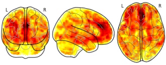
The following inclusion criteria were applied to the database of 113 studies: 1) gray matter VBM study comparing adult patients with PTSD to either non-traumatised-controls or traumatised-controls; 2) results presented in Talairach or MNI coordinates; 3) studies were only included if a whole brain analysis was performed rather than a small volume correction to ensure no bias in the regions reported. Thirteen studies met inclusion criteria and are listed in Table S1. We emailed all study authors who used SPM (Statistical Parametric Mapping) to process their data for a ‘T-map’ image comparing PTSD gray matter volume to the control group. ‘T-maps’ are three dimensional maps comprising statistical data of volume differences in thousands of voxels in the brain and provide far more detailed information than significant coordinates reported in studies. However, SDM allows both T-maps and coordinates to be combined in a single meta-analysis and the methodology reported in detail by Radua et al. We received 6 T-maps from 6 independent studies and these were included in the meta-analyses. In addition to the main meta-analysis comparing PTSD to all controls, three additional VBM analyses were conducted: 1) comparing the PTSD group with non-traumatised-controls only 2) comparing the PTSD group with traumatised-controls only, 3) comparing PTSD group with all controls and widening the criteria to include paediatric studies. T-maps and coordinates signifying gray matter volume changes from where we were unable to obtain T-maps were extracted from relevant studies and analysed using Seed-based d Mapping (SDM version 5.14, http://www.sdmproject.com). For studies where coordinate data was used, these were convolved with a Gaussian kernel (FWHM=20mm) in order to optimally compensate the sensitivity and specificity of the analysis. As is standard in SDM analyses, the number of randomizations were set to 100 and a threshold was set at p<0.005 as well as a cluster-level threshold of 10 voxels in order to increase sensitivity and correctly control false-positive rate.8 A jackknife sensitivity analysis was performed in order to assess the robustness of the results which was achieved by excluding one study in each of the analyses.

Collection description

OBJECTIVE:
The authors conducted a comprehensive meta-analysis of MRI region-of-interest and voxel-based morphometry (VBM) studies in posttraumatic stress disorder (PTSD). Because patients have high rates of comorbid depression, an additional objective was to compare the findings to a meta-analysis of MRI studies in depression.

METHOD:
The MEDLINE database was searched for studies from 1985 through 2016. A total of 113 studies met inclusion criteria and were included in an online database. Of these, 66 were selected for the region-of-interest meta-analysis and 13 for the VBM meta-analysis. The region-of-interest meta-analysis was conducted and compared with a meta-analysis of major depressive disorder. Within the region-of-interest meta-analysis, three subanalyses were conducted that included control groups with and without trauma.

RESULTS:
In the region-of-interest meta-analysis, patients with PTSD compared with all control subjects were found to have reduced brain volume, intracranial volume, and volumes of the hippocampus, insula, and anterior cingulate. PTSD patients compared with nontraumatized or traumatized control subjects showed similar changes. Traumatized compared with nontraumatized control subjects showed smaller volumes of the hippocampus bilaterally. For all regions, pooled effect sizes (Hedges' g) varied from -0.84 to 0.43, and number of studies from three to 41. The VBM meta-analysis revealed prominent volumetric reductions in the medial prefrontal cortex, including the anterior cingulate. Compared with region-of-interest data from patients with major depressive disorder, those with PTSD had reduced total brain volume, and both disorders were associated with reduced hippocampal volume.

CONCLUSIONS:
The meta-analyses revealed structural brain abnormalities associated with PTSD and trauma and suggest that global brain volume reductions distinguish PTSD from major depression.

Subject species

homo sapiens

Modality

Structural MRI

Analysis level

meta-analysis

Cognitive paradigm (task)

2nd-order rule acquisition

Map type

Z

Depression Therapeutics Market Outlook

According to our latest research, the global depression therapeutics market size reached USD 16.4 billion in 2024, reflecting the increasing prevalence of depressive disorders and the growing demand for innovative treatment solutions. The market is expected to expand at a robust CAGR of 6.2% between 2025 and 2033, ultimately reaching a forecasted value of USD 28.1 billion by 2033. This growth is primarily driven by the rising diagnosis rates, expanding access to mental health services, and the introduction of novel therapeutic modalities targeting treatment-resistant depression, as per our comprehensive analysis of the latest industry data.

One of the most significant growth factors propelling the depression therapeutics market is the global surge in mental health awareness initiatives, which have substantially reduced the stigma surrounding depressive disorders. Public health campaigns, educational programs, and advocacy by non-governmental organizations have collectively improved recognition of depression symptoms and encouraged more individuals to seek professional help. This heightened awareness has led to a notable increase in the diagnosis and treatment of depression, thereby escalating the demand for both pharmacological and non-pharmacological interventions. Furthermore, the proliferation of digital health platforms and telemedicine services has made mental health resources more accessible, particularly in remote and underserved regions, further expanding the patient pool eligible for depression therapeutics.

Another critical driver of market growth is the continuous innovation in drug development, particularly the advent of next-generation antidepressants and adjunctive therapies. Pharmaceutical companies are increasingly investing in research and development to address the limitations of existing medications, such as delayed onset of action, side effects, and inadequate response rates in certain patient populations. Notably, the approval and commercialization of novel agents like esketamine and digital therapeutics have expanded the therapeutic arsenal for clinicians treating major depressive disorder and treatment-resistant depression. Additionally, there is a growing emphasis on personalized medicine, with genetic testing and biomarker-based approaches enabling the selection of optimal therapeutic regimens tailored to individual patient profiles, thereby improving treatment efficacy and patient outcomes.

The integration of multidisciplinary treatment modalities, including pharmacotherapy, psychotherapy, and neuromodulation techniques, has also significantly contributed to the expansion of the depression therapeutics market. Healthcare providers increasingly recognize the importance of a holistic approach to managing depression, combining medication with evidence-based psychotherapies such as cognitive behavioral therapy (CBT) and emerging interventions like transcranial magnetic stimulation (TMS) and electroconvulsive therapy (ECT). This integrated care model not only enhances treatment effectiveness but also addresses comorbid conditions, such as anxiety and substance use disorders, which frequently coexist with depression. The growing adoption of such comprehensive treatment strategies is expected to sustain market growth over the coming years.

Regionally, North America continues to dominate the depression therapeutics market, accounting for the largest share in 2024, followed by Europe and Asia Pacific. The high prevalence of depressive disorders, well-established healthcare infrastructure, and favorable reimbursement policies in North America have contributed to its leadership position. However, the Asia Pacific region is poised for the fastest growth, driven by increasing mental health awareness, expanding healthcare spending, and ongoing investments in mental health infrastructure. Latin America and the Middle East & Africa are also witnessing gradual improvements in depression management, although challenges related to stigma and limited access to care persist in certain countries.

Drug Class Analysis</h2

The Survey of Consumer Attitudes and Behavior series (also known as the Surveys of Consumers) was undertaken to measure changes in consumer attitudes and expectations, to understand why such changes occur, and to evaluate how they relate to consumer decisions to save, borrow, or make discretionary purchases. The data regularly include the Index of Consumer Sentiment, the Index of Current Economic Conditions, and the Index of Consumer Expectations. Since the 1940s, these surveys have been produced quarterly through 1977 and monthly thereafter. The surveys conducted in 2010 focused on topics such as evaluations and expectations about personal finances, employment, price changes, and the national business situation. Opinions were collected regarding respondents' appraisals of present market conditions for purchasing houses, automobiles, and other durables. Explored in this survey were respondents' types of savings and financial investments, loan use, family income, and retirement planning. This survey also asked respondents about financial and health literacy; adult and online education; and technology use in health, finances, travel, and communication. Additional questions on independent living communities and general feelings were asked. Other topics in this series typically include ownership, lease, and use of automobiles, respondents' use of personal computers at home and in the office, and respondents' familiarity with and use of the Internet. Demographic information include ethnic origin, sex, age, marital status, and education.

Anthropogenically fragmented populations may have reduced fitness due to loss of genetic diversity and inbreeding. The extent of such fitness losses due to fragmentation and potential gains from conservation actions are infrequently assessed together empirically. Controlled crosses within and among populations can identify whether populations are at risk of inbreeding depression and whether interpopulation crossing alleviates fitness loss. Because fitness depends on environment and life stage, studies quantifying cumulative fitness over a large portion of the lifecycle in conditions that mimic natural environments are most informative. To assess fitness consequences of habitat fragmentation, we leveraged controlled within-family, within-population, and between-population crosses to quantify inbreeding depression and heterosis in seven populations of Echinacea angustifolia within a 6400-hectare area. We then assessed cumulative offspring fitness after 14 years of growth in a natural experimental plot (N = 1136). Mean fitness of progeny from within-population crosses varied considerably, indicating genetic differentiation among source populations, even though these sites are all less than 9 km apart. The fitness consequences of within-family and between-population crosses varied in magnitude and direction. Only one of the seven populations showed inbreeding depression of high effect, while four populations showed substantial heterosis. Outbreeding depression was rare and slight. Our findings indicate that local crossings between isolated populations yield unpredictable fitness consequences ranging from slight decreases to substantial increases. Interestingly, inbreeding depression and heterosis did not relate closely to population size, suggesting that all fragmented populations could contribute to conservation goals as either pollen recipients or donors. Methods We performed controlled within-family, within-population, and between-population crosses of the prairie perennial, Echinacea angustifolia (Asteraceae) originating from seven remnant populations. We then assessed the cumulative fitness of progeny over 14 years in an experimental plot using aster models.

The Volcker Shock was a period of historically high interest rates precipitated by Federal Reserve Chairperson Paul Volcker's decision to raise the central bank's key interest rate, the Fed funds effective rate, during the first three years of his term. Volcker was appointed chairperson of the Fed in August 1979 by President Jimmy Carter, as replacement for William Miller, who Carter had made his treasury secretary. Volcker was one of the most hawkish (supportive of tighter monetary policy to stem inflation) members of the Federal Reserve's committee, and quickly set about changing the course of monetary policy in the U.S. in order to quell inflation. The Volcker Shock is remembered for bringing an end to over a decade of high inflation in the United States, prompting a deep recession and high unemployment, and for spurring on debt defaults among developing countries in Latin America who had borrowed in U.S. dollars.

Monetary tightening and the recessions of the early '80s

Beginning in October 1979, Volcker's Fed tightened monetary policy by raising interest rates. This decision had the effect of depressing demand and slowing down the U.S. economy, as credit became more expensive for households and businesses. The Fed funds rate, the key overnight rate at which banks lend their excess reserves to each other, rose as high as 17.6 percent in early 1980. The rate was allowed to fall back below 10 percent following this first peak, however, due to worries that inflation was not falling fast enough, a second cycle of monetary tightening was embarked upon starting in August of 1980. The rate would reach its all-time peak in June of 1981, at 19.1 percent. The second recession sparked by these hikes was far deeper than the 1980 recession, with unemployment peaking at 10.8 percent in December 1980, the highest level since The Great Depression. This recession would drive inflation to a low point during Volcker's terms of 2.5 percent in August 1983.

The legacy of the Volcker Shock

By the end of Volcker's terms as Fed Chair, inflation was at a manageable rate of around four percent, while unemployment had fallen under six percent, as the economy grew and business confidence returned. While supporters of Volcker's actions point to these numbers as proof of the efficacy of his actions, critics have claimed that there were less harmful ways that inflation could have been brought under control. The recessions of the early 1980s are cited as accelerating deindustrialization in the U.S., as manufacturing jobs lost in 'rust belt' states such as Michigan, Ohio, and Pennsylvania never returned during the years of recovery. The Volcker Shock was also a driving factor behind the Latin American debt crises of the 1980s, as governments in the region defaulted on debts which they had incurred in U.S. dollars. Debates about the validity of using interest rate hikes to get inflation under control have recently re-emerged due to the inflationary pressures facing the U.S. following the Coronavirus pandemic and the Federal Reserve's subsequent decision to embark on a course of monetary tightening.