The use of linked data research in UK decision-making related to early life...
- figshare.com
xlsxUpdated Sep 7, 2023+ more versions Share
Share Facebook
 Twitter
 EmailClick to copy linkLink copiedCiteHollie Henderson (2023). The use of linked data research in UK decision-making related to early life health: A Systematic Map (Supplementary Material) [Dataset]. http://doi.org/10.6084/m9.figshare.24006906.v1xlsxAvailable download formatsUnique identifierhttps://doi.org/10.6084/m9.figshare.24006906.v1Dataset updatedSep 7, 2023AuthorsHollie HendersonLicense
Attribution 4.0 (CC BY 4.0)https://creativecommons.org/licenses/by/4.0/
License information was derived automaticallyArea coveredUnited KingdomDescriptionA systematic mapping review was conducted with the aim of providing an overall description of how linked data research has been used in UK decision-making relating to early life health; exploring the factors affecting the use of linked data as evidence in these decisions; and identifying where evidence gaps to inform further research.This mapping review forms part of a PhD project being undertaken by Hollie Henderson at the University of York, which aims to understand how linked data can be used as a local health intelligence tool for child and maternal health. This project is funded by the White Rose Consortium and is part of the National Institute for Health Research (NIHR) Yorkshire and Humber Applied Research Collaboration (YHARC).This document presents the Systematic Map that is associated with this mapping review.
1897-1907 Bartholomew historic map
- arcgis.com
- hub.arcgis.com
Updated Apr 26, 2018+ more versionsShareFacebookTwitterEmailClick to copy linkLink copiedCiteEsri UK Education (2018). 1897-1907 Bartholomew historic map [Dataset]. https://www.arcgis.com/sharing/oauth2/social/authorize?socialLoginProviderName=google&oauth_state=a5jhUklb9BFQ_thoRpy9uYg..wQbhmhnffnk-5Y3uGhd4Xeiru47hz9tsX9fsHfQ653gb9cHqBgOeOxYNkkt_5b-gVaaYi9PNYmJgMa-5otlRvptpR-Mr-i5og_AC2coccANiAsBXMxz_P3IZ9nH0QxiUgRPLfh8vQlewCHuwY0q2FE5d_VkTWNkab34CiABZatKdttRL52HKc_WDNFsEZvfU40qMsKhuEbaTIHUY0TjSp_bnGOsNxVC70jF4498LGjbL21apjYOKxTzz3yKVwNY5RX1jjPIMF9PoeH5FgcBXc81QWdXravWKV99B8gsqblNLEuU-H38LWrN9abupD-u3pEc2Ojeg62aMf5ClzQrqy-OIjThJy0WV42h3Dataset updatedApr 26, 2018AuthorsEsri UK EducationArea coveredDescriptionColourful and easy to use, Bartholomew’s maps became a trademark series. The maps were popular and influential, especially for recreation, and the series sold well, particularly with cyclists and tourists. To begin with, Bartholomew printed their half-inch maps in Scotland as stand-alone sheets known as 'District Sheets' and by 1886 the whole of Scotland was covered. They then revised the maps into an ordered set of 29 sheets covering Scotland in a regular format. This was first published under the title Bartholomew’s Reduced Ordnance Survey of Scotland. The half-inch maps of Scotland formed the principal content for Bartholomew's Survey Atlas of Scotland published in 1895. Bartholomew then moved south of the Border to the more lucrative but competitive market in England and Wales, whilst continuing to revise the Scottish sheets. The first complete coverage of Great Britain at the half-inch scale was achieved by 1903, and this is the layer shown here.The half-inch maps were distinctive for using different layers of colour to represent landscape relief. A subtle and innovative gradation of colour bands were employed for land at different heights. Lighter greens were used for low ground closest to sea-level, darker greens and browns for higher ground, with white used for mountain tops. Whilst layer colouring had been developed in Germany from the 1860s, Bartholomew's development of it was both innovative and influential. John Bartholomew junior (1831-1893) first used the firm's trademark layer colouring in Baddeley’s Thorough Guide to the English Lake District (1880). His son, John George Bartholomew (1860-1920), later went on to refine the style. You can see Bartholomew’s continued experimentation with layer colour palettes in the Cairngorms layer colour explorer ( http://geo.nls.uk/maps/bartholomew/layers/ )
Bartholomew based their half-inch maps on more detailed Ordnance Survey mapping at one-inch to the mile (1:63,360). The firm had published 'Reduced Ordnance Maps' of Scotland, England and Wales at this scale from the 1890s. These maps were progressively revised and updated with new information. Usually Bartholomew made revisions the sheets right up to the time of publication, so the date of publication is the best guide to the approximate date of the features shown on the map. You can view the dates of publication for the series at:
● Scotland: https://maps.nls.uk/series/bart_half_scotland.html
● England and Wales: https://maps.nls.uk/series/bart_half_england.html
- n
Whites Vegetation Map
- cmr.earthdata.nasa.gov
Updated Apr 21, 2017+ more versionsShareFacebookTwitterEmailClick to copy linkLink copiedCite(2017). Whites Vegetation Map [Dataset]. https://cmr.earthdata.nasa.gov/search/concepts/C1214599913-SCIOPSDataset updatedApr 21, 2017Time period coveredJan 1, 2000 - Dec 31, 2000DescriptionThe Vegetation Map of Africa is a compendium of various existing map sources for different regions/countries, which were integrated and synthesized by the AETFAT committeee responsible for creating the map (headed by Dr. F. White of Oxford University, UK). The first draft of the map was checked by extensive fieldwork and discussions with local experts. The vegetation classification used is the UNESCO standard based on physiognomy and floristic composition (not climate), and it includes a total of 80 major vegetation types and mosaics. Water is added as category 81 in the GRID legend for the digital map.
Population of the UK 2023, by region
- statista.com
- ai-chatbox.pro
Updated Oct 14, 2024ShareFacebookTwitterEmailClick to copy linkLink copiedCiteStatista (2024). Population of the UK 2023, by region [Dataset]. https://www.statista.com/statistics/294729/uk-population-by-region/Dataset updatedOct 14, 2024Time period covered2023Area coveredUnited KingdomDescriptionThe population of the United Kingdom in 2023 was estimated to be approximately 68.3 million in 2023, with almost 9.48 million people living in South East England. London had the next highest population, at over 8.9 million people, followed by the North West England at 7.6 million. With the UK's population generally concentrated in England, most English regions have larger populations than the constituent countries of Scotland, Wales, and Northern Ireland, which had populations of 5.5 million, 3.16 million, and 1.92 million respectively. English counties and cities The United Kingdom is a patchwork of various regional units, within England the largest of these are the regions shown here, which show how London, along with the rest of South East England had around 18 million people living there in this year. The next significant regional units in England are the 47 metropolitan and ceremonial counties. After London, the metropolitan counties of the West Midlands, Greater Manchester, and West Yorkshire were the biggest of these counties, due to covering the large urban areas of Birmingham, Manchester, and Leeds respectively. Regional divisions in Scotland, Wales and Northern Ireland The smaller countries that comprise the United Kingdom each have different local subdivisions. Within Scotland these are called council areas whereas in Wales the main regional units are called unitary authorities. Scotland's largest Council Area by population is that of Glasgow City at over 622,000, while in Wales, it was the Cardiff Unitary Authority at around 372,000. Northern Ireland, on the other hand, has eleven local government districts, the largest of which is Belfast with a population of around 348,000.
- b
Geological Map of the Gwasi Area (Black and white)
- hosted-metadata.bgs.ac.uk
jpgUpdated 1954ShareFacebookTwitterEmailClick to copy linkLink copiedCiteMinistry of Petroleum and Mining (National Geodata Centre for Kenya) (1954). Geological Map of the Gwasi Area (Black and white) [Dataset]. https://hosted-metadata.bgs.ac.uk/geonetwork/srv/api/records/07a139cd-53c1-4679-850b-7147ad79995d?language=alljpgAvailable download formatsDataset updated1954Dataset provided byMinistry of Petroleum and Mining (National Geodata Centre for Kenya)Area coveredDescriptionDegree Sheet: 61 SE, Sheet Number (Directorate of Overseas Survey): 186, Report: Not applicable
- N
Meta-analysis of regional white matter volume in bipolar disorder with...
- neurovault.org
niftiUpdated Jun 30, 2018+ more versionsShareFacebookTwitterEmailClick to copy linkLink copiedCite(2018). Meta-analysis of regional white matter volume in bipolar disorder with replication in an independent sample using coordinates, T-maps, and individual MRI data: Independent study for replication Gray matter (contrast = Control > Patients so positives values are reduction in volume) [Dataset]. http://identifiers.org/neurovault.image:61001niftiAvailable download formatsUnique identifierhttps://identifiers.org/neurovault.image:61001Dataset updatedJun 30, 2018LicenseCC0 1.0 Universal Public Domain Dedicationhttps://creativecommons.org/publicdomain/zero/1.0/
License information was derived automaticallyDescriptionDetails from paper:
Subjects
The VBM analysis included 26 euthymic patients with BD (23 with bipolar I and 3 with bipolar II, 9 males and 17 females) and 23 healthy control subjects (7 males and 16 females). The patients were primarily recruited from a UK patient support group, healthy controls were recruited via advertisements in local media. The study was approved by the local ethics committee and written informed consent was obtained from all participants. All subjects were assessed using the Structural Clinical Interview for DSM-IV Axis I Disorders (SCID-CV). Patients were included if they fulfilled criteria for DSM-IV for BD and did not have any comorbidity for other DSM-IV Axis-I disorders. Healthy controls subjects were selected in order to match BD patients for age, sex, race/ethnicity, weight, height, handedness, premorbid IQ, years of education, lifetime drug and alcohol use. They were included if they had no DSM-IV Axis I disorders and no family history of psychiatric conditions. The mean age was 42.1 (± SD 14.8) for BD patients and 41.2 (± SD 14.0) for healthy controls. Demographic and clinical measures are given in table s1 and s2.MRI acquisition
Participants were scanned using a 1.5 Tesla Siemens Magnetom Vision MRI scanner to obtain T1 weighted MPRAGE (Multi-Planar Rapidly Acquired Gradient Echo) scans. In order to confer good resolution and good contrast between grey and white matter in particular, the following parameters were selected: TR = 9.7 ms, TE = 4 ms, TI = 300 ms, Nex = 1, 256 x 192 matrix, flip angle = 8°, 128 slices, voxel size = 1.0 x 1.0 x 2.0mm. There was no significant difference in scan date between patients and controls (p=0.28).VBM DARTEL pre-processing
We examined group-related differences in regional brain volume using voxel-based morphometry, as implemented in SPM8 software (http://www.fil.ion.ucl.ac.uk/spm/) running under MATLAB R2012b, version 8.0 (The MathWorks, Icn, Natick, Massachussetts). First the T1-weighted images were pre-processed using the DARTEL (Diffeomorphic Anatomical Registration using Exponentiated Lie algebra) algorithm (Ashburner, 2007) following the steps described by Ashburner (Ashburner, 2010). Firstly, each T1-weighted image was checked for scanner artefacts and gross anatomical abnormalities and then manually reoriented to the Anterior Commissure-Posterior Commissure line blind to diagnosis. The images were then segmented into grey matter, white matter and cerebrospinal fluid in native space. The DARTEL SPM8 toolbox was used to implement the high-dimensional DARTEL normalization through which the DARTEL template was created from the images of all the subjects of the study. During the template creation, flow fields were computed which contain information about the transformation from every native image to the DARTEL template (Peelle et al., 2012). This procedure increases the accuracy of the alignment between subjects by using millions of parameters to characterise the spatial transformations of each brain (Ashburner, 2010). In order to allow for inter-study comparisons, the segmented images were spatially normalized to MNI space including the flow fields in the process. The images were ‘modulated’ to conserve the information on absolute volume. Smoothing was applied to the images using a FWHM 8mm isotropic Gaussian kernel resulting in smoothed, segmented, normalized, and modulated images.VBM Statistical analysis
A central aim of the study was to examine the volume of the white matter ROI created by the meta-analysis in an independent sample, however for completeness in the supplementary materials we present the whole VBM brain analysis of the independent dataset. Total intracranial volume was determined for each subject by summing grey matter, white matter and CSF segmentations. The regional differences in voxel-based parameters between BD and controls were assessed using a General Linear Model (GLM) with total intracranial volume and age as covariates of no interest. An absolute threshold masking of 0.05 was adopted in order to exclude voxels outside the brain. A height threshold of p < 0.05 FWE (family wise error) corrected was initially adopted to detect significant regional differences. In addition a more liberal height threshold of p < 0.001, uncorrected for multiple comparisons, was also applied with a cluster threshold of 10 voxels. Following this height threshold, a non-stationary cluster extend correction was implemented at the cluster threshold of p < 0.05 family-wise error (FWE) corrected for multiple comparisons in order to account for the non-isotropic (non-uniform) smoothness across the data (Hayasaka et al., 2004; Worsley et al., 1999). This correction was performed using the VBM8 toolbox (available online at http://dbm.neuro.uni-jena.de/vbm/download). Finally we implemented the same method excluding patients who were taking lithium as studies have demonstrated that lithium may increase total grey matter volume (Hallahan et al., 2011; Kempton et al., 2008; Monkul et al., 2007; Moore et al., 2009; Sassi et al., 2002). Montreal Neurological Institute (MNI) coordinates are reported in the results tables (supplementary table 3 and table 4), however these coordinates were converted to Talairach coordinates to determine the names of corresponding brain regions. MNI coordinates were converted to Talairach using GingerALE, version 2.1.1 (available online at http://www.brainmap.org/ale/) and brain region names were determined using Talairach Client, version 2.4.3 (available online at http://www.talairach.org/client.html).Supplementary Results
Independent VBM whole brain study results
No significant differences in white or gray matter volume were found at the height threshold of p < 0.05 FWE corrected. The analysis was then repeated with a height threshold of p < 0.001 uncorrected. Regions of significant white matter volume decreases at a height threshold of p<0.001 uncorrected are shown in supplementary table 3. No regions of significant increased white matter in bipolar patients compared to controls were found. Two clusters of voxels survived the additional non-stationary cluster extent threshold of p < 0.05 FWE corrected for multiple comparisons in the white matter results. These clusters encompassed white matter adjacent to the cingulate gyrus and in the corpus callosum (supplementary figure 3). Grey matter volume differences between the two groups are also shown in supplementary table 3. Finally, we found regions of decreased and increased grey matter in bipolar patients that were not taking lithium compared to healthy controls (supplementary table 4). The T-maps of each contrast are freely available to download from www.bipolardatabase.org. The white matter results have been used in the main paper to validate the region of interest found in our meta-analysis.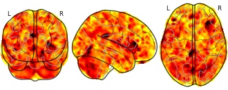
Collection description
Converging evidence suggests that bipolar disorder (BD) is associated with white matter (WM) abnormalities.
Meta-analyses of voxel based morphometry (VBM) data is commonly performed using published coordinates,
however this method is limited since it ignores non-significant data. Obtaining statistical maps from studies (Tmaps)
as well as raw MRI datasets increases accuracy and allows for a comprehensive analysis of clinical
variables. We obtained coordinate data (7-studies), T-Maps (12-studies, including unpublished data) and raw
MRI datasets (5-studies) and analysed the 24 studies using Seed-based d Mapping (SDM). A VBM analysis was
conducted to verify the results in an independent sample. The meta-analysis revealed decreased WM volume in
the posterior corpus callosum extending to WM in the posterior cingulate cortex. This region was significantly
reduced in volume in BD patients in the independent dataset (p = 0.003) but there was no association with
clinical variables. We identified a robust WM volume abnormality in BD patients that may represent a trait
marker of the disease and used a novel methodology to validate the findingsSubject species
homo sapiens
Modality
Structural MRI
Analysis level
group
Cognitive paradigm (task)
Young Mania Rating Scale
Map type
T
- b
Geological Map of the Kilifi Mazeras Area (Black and white)
- hosted-metadata.bgs.ac.uk
jpgUpdated 1952ShareFacebookTwitterEmailClick to copy linkLink copiedCiteMinistry of Petroleum and Mining (National Geodata Centre for Kenya) (1952). Geological Map of the Kilifi Mazeras Area (Black and white) [Dataset]. https://hosted-metadata.bgs.ac.uk/geonetwork/srv/api/records/fff9f4e6-4182-424a-b2d9-293ed66fed66?language=alljpgAvailable download formatsDataset updated1952Dataset provided byMinistry of Petroleum and Mining (National Geodata Centre for Kenya)Area coveredDescriptionDegree Sheet: 66 SE, Sheet Number (Directorate of Overseas Survey): Not applicable, Report: Not applicable
- b
Ministry of Petroleum and Mining (National Geodata Centre for Kenya)
- hosted-metadata.bgs.ac.uk
jpgUpdated 1945ShareFacebookTwitterEmailClick to copy linkLink copiedCiteMinistry of Petroleum and Mining (National Geodata Centre for Kenya) (1945). Ministry of Petroleum and Mining (National Geodata Centre for Kenya) [Dataset]. https://hosted-metadata.bgs.ac.uk/geonetwork/srv/api/records/3458aa5f-1dd1-4d4b-b171-649a6b4e5c0fjpgAvailable download formatsDataset updated1945Dataset provided byMinistry of Petroleum and Mining (National Geodata Centre for Kenya)Area coveredDescriptionDegree Sheet: 43 NE, Sheet Number (Directorate of Overseas Survey): Not applicable, Report: Not applicable
Mineral Resource Polygons Northern Ireland (Internal Geological Boundaries...
- data.europa.eu
- metadata.bgs.ac.uk
- +2more
html, unknownUpdated Oct 11, 2021+ more versionsShareFacebookTwitterEmailClick to copy linkLink copiedCiteBritish Geological Survey (BGS) (2021). Mineral Resource Polygons Northern Ireland (Internal Geological Boundaries Retained) [Dataset]. https://data.europa.eu/data/datasets/mineral-resource-polygons-northern-ireland-internal-geological-boundaries-retainedhtml, unknownAvailable download formatsDataset updatedOct 11, 2021AuthorsBritish Geological Survey (BGS)Area coveredIreland, Northern IrelandDescriptionThis mineral resource data was produced as part of the Mineral Resource Map of Northern Ireland via a commission from the Northern Ireland Department of the Environment. The work resulted in a series of 21 data layers which were used to generate a series of six digitally generated maps. This work was completed in 2012 with one map for each of the six counties (including county boroughs) of Northern Ireland at a scale of 1:100 000. This data and the accompanying maps are intended to assist strategic decision making in respect of mineral extraction and the protection of important mineral resources against sterilisation. They bring together a wide range of information, much of which is scattered and not always available in a convenient form. The data has been produced by the collation and interpretation of mineral resource data principally held by the Geological Survey of Northern Ireland and was funded via a commission from the Northern Ireland Department of the Environment. These layers display the spatial data of the mineral resources of Northern Ireland. There are a series of layers which consist of: Bedrock: Clay, Bauxitic clay, Coal & Lignite, Coal – lignite proven, Conglomerate, Dolomite, Igneous and meta-igneous rock, Limestone, a 100m buffer layer on the Ulster White Limestone, Meta-sedimentary rocks, Perlite, Salt, Sandstone and Silica Sand. Superficial (unconsolidated recent sediments) : Sand & gravel and Peat. The data except for the salt and proven lignite resource layers was derived from the 1:50 00 and 1:250 000 scale DigMap NI dataset. This version of the data retains the internal geological boundaries which are dissolved out in the accompanying dissolved version. A user guide 'The Mineral Resources of Northern Ireland digital dataset (version 1)' OR/12/039 describing the creation and use of the data is available.
- b
Mombasa Kwale Area (black and white sketch maps)
- hosted-metadata.bgs.ac.uk
jpgUpdated Oct 22, 2019ShareFacebookTwitterEmailClick to copy linkLink copiedCiteMinistry of Petroleum and Mining (National Geodata Centre for Kenya) (2019). Mombasa Kwale Area (black and white sketch maps) [Dataset]. https://hosted-metadata.bgs.ac.uk/geonetwork/srv/api/records/fdd01c85-905e-4136-aeda-8dfc9e0541f7?language=alljpgAvailable download formatsDataset updatedOct 22, 2019Dataset provided byMinistry of Petroleum and Mining (National Geodata Centre for Kenya)Area coveredKwale County, MombasaDescriptionDegree Sheet: 69, Sheet Number (Directorate of Overseas Survey): Not applicable, Report: 24
- b
Geological Map of the Magadi Area(black and white)
- hosted-metadata.bgs.ac.uk
jpgUpdated 1952ShareFacebookTwitterEmailClick to copy linkLink copiedCiteMinistry of Petroleum and Mining (National Geodata Centre for Kenya) (1952). Geological Map of the Magadi Area(black and white) [Dataset]. https://hosted-metadata.bgs.ac.uk/geonetwork/srv/api/records/0e77ed5b-5b86-480c-b18d-4d5daa895d94jpgAvailable download formatsDataset updated1952Dataset provided byMinistry of Petroleum and Mining (National Geodata Centre for Kenya)Area coveredDescriptionDegree Sheet: 51 SW, Sheet Number (Directorate of Overseas Survey): 160, Report: Not applicable
- b
Geological Map of the Kakamega Area (Black and white)
- hosted-metadata.bgs.ac.uk
jpgUpdated 1953ShareFacebookTwitterEmailClick to copy linkLink copiedCiteMinistry of Petroleum and Mining (National Geodata Centre for Kenya) (1953). Geological Map of the Kakamega Area (Black and white) [Dataset]. https://hosted-metadata.bgs.ac.uk/geonetwork/srv/api/records/eacb5d71-92ec-432e-a581-2b5deed87c0fjpgAvailable download formatsDataset updated1953Dataset provided byMinistry of Petroleum and Mining (National Geodata Centre for Kenya)Area coveredDescriptionDegree Sheet: 33 SE, Sheet Number (Directorate of Overseas Survey): Not applicable, Report: Not applicable
- N
Exploring white matter microstructure and the impact of antipsychotics in...
- neurovault.org
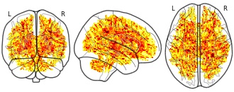
niftiUpdated May 15, 2020+ more versionsShareFacebookTwitterEmailClick to copy linkLink copiedCite(2020). Exploring white matter microstructure and the impact of antipsychotics in adolescent-onset psychosis: FA map, contrast patients > controls (unthresholded t map) [Dataset]. http://identifiers.org/neurovault.image:387082niftiAvailable download formatsUnique identifierhttps://identifiers.org/neurovault.image:387082Dataset updatedMay 15, 2020LicenseCC0 1.0 Universal Public Domain Dedicationhttps://creativecommons.org/publicdomain/zero/1.0/
License information was derived automaticallyDescriptionFor contrasting case-control differences, we run voxel-wise statistics for FA using a nonparametric permutation-based approach (FSL, Randomise, 5000 permutations). Age and sex were entered as covariates. All covariates were demeaned. The map shows uncorrected test statistic (see https://fsl.fmrib.ox.ac.uk/fsl/fslwiki/Randomise/UserGuide).
Collection description
Unthresholded t- and corrected p-maps of the scalar diffusion measures fractional anistropy (FA), axial diffusivity (AD) and radial diffusivity (RD), contrasting adolescent patients with early onset psychosis versus adolescent healthy controls (i.e. contrast 1: patients >controls; contrast 2: patients > controls, covariates: age and sex).
Preprint: https://www.biorxiv.org/content/10.1101/721225v2
Subject species
homo sapiens
Modality
Diffusion MRI
Analysis level
group
Cognitive paradigm (task)
None / Other
Map type
T
- E
Cover of Land Cover Map 2007 broad habitat classes in the upstream catchment...
- catalogue.ceh.ac.uk
- hosted-metadata.bgs.ac.uk
- +1more
csvUpdated Jun 26, 2017+ more versionsShareFacebookTwitterEmailClick to copy linkLink copiedCiteJ. Murphy; T. Oliver (2017). Cover of Land Cover Map 2007 broad habitat classes in the upstream catchment of the 20 Wessex chalkstream sites, England, UK [Dataset]. http://doi.org/10.5285/b8a66584-da67-49e5-a0b0-d8e0b3e75b99csvAvailable download formatsUnique identifierhttps://doi.org/10.5285/b8a66584-da67-49e5-a0b0-d8e0b3e75b99Dataset updatedJun 26, 2017Dataset provided byNERC EDS Environmental Information Data CentreAuthorsJ. Murphy; T. OliverTime period coveredJan 1, 2012 - Dec 31, 2012Area coveredDescriptionThe data consists of a matrix of twelve land cover classes by 20 stream sites with the area of each land cover class given in km^2. The areal coverage (km2) of each of twelve land cover classes was recorded for each of 20 chalkstream catchments in southern England. The 20 discrete chalkstream catchments are distributed along the white chalk geology extending from Dorset in the south west, through Wiltshire, to Hampshire in the north east, to cover a gradient of catchment land cover intensification from extensive calcareous grassland and woodland through to arable and improved grasslands. These data were acquired in July 2012. This dataset was created as part of work package 3.1 of the Wessex Biodiversity & Ecosystem Service Sustainability (BESS) project.
Early Miocene ASEM element maps from IODP Site U1480 (NERC grant...
- data-search.nerc.ac.uk
- metadata.bgs.ac.uk
- +1more
htmlUpdated Apr 16, 2019ShareFacebookTwitterEmailClick to copy linkLink copiedCiteUniversity of Cardiff (2019). Early Miocene ASEM element maps from IODP Site U1480 (NERC grant NE/P021182/1) [Dataset]. https://data-search.nerc.ac.uk/geonetwork/srv/api/records/823bd11c-b7a6-6aa5-e054-002128a47908htmlAvailable download formatsDataset updatedApr 16, 2019AuthorsUniversity of CardiffLicensehttp://inspire.ec.europa.eu/metadata-codelist/LimitationsOnPublicAccess/noLimitationshttp://inspire.ec.europa.eu/metadata-codelist/LimitationsOnPublicAccess/noLimitations
Time period coveredFeb 1, 2018 - Jul 1, 2018Area coveredDescriptionElement maps from 5x 10 cm sections generated using the Zeiss Sigma HD Field Emission Gun Analytical SEM at Cardiff University. Maps come from sections within the early Miocene pelagic interval situated directly below the Nicobar Fan succession at IODP Site U1480 in the Eastern Equatorial Indian Ocean (for more information see published report, https://doi.org/10.1016/j.epsl.2017.07.019). These specific sections were chosen to examine the depositional environments associated with transitions from red clays to white chalk, which demonstrate distinct banding at the micro and macro scale.
- b
Geological Map of the Sultan Hamud Area (Black and white)
- hosted-metadata.bgs.ac.uk
jpgUpdated 1954ShareFacebookTwitterEmailClick to copy linkLink copiedCiteMinistry of Petroleum and Mining (National Geodata Centre for Kenya) (1954). Geological Map of the Sultan Hamud Area (Black and white) [Dataset]. https://hosted-metadata.bgs.ac.uk/geonetwork/srv/api/records/cfb45e9a-1c73-4907-986f-30826d74f0e6jpgAvailable download formatsDataset updated1954Dataset provided byMinistry of Petroleum and Mining (National Geodata Centre for Kenya)Area coveredDescriptionDegree Sheet: 59 NW, Sheet Number (Directorate of Overseas Survey): Not applicable, Report: Not applicable
- d
Great Crested Newt - Risk Zones (Derbyshire)
- environment.data.gov.uk
Updated Mar 14, 2021+ more versionsShareFacebookTwitterEmailClick to copy linkLink copiedCiteNatural England (2021). Great Crested Newt - Risk Zones (Derbyshire) [Dataset]. https://environment.data.gov.uk/dataset/8ed925cd-0270-48a1-9d2c-146e34c1a171Dataset updatedMar 14, 2021Licensehttps://www.gov.uk/government/publications/natural-englands-maps-and-data-terms-of-use/terms-of-use-for-natural-englands-maps-and-datahttps://www.gov.uk/government/publications/natural-englands-maps-and-data-terms-of-use/terms-of-use-for-natural-englands-maps-and-data
Area coveredDerbyshireDescriptionThis dataset identifies areas where the distribution of great crested newts (GCN) has been categorised into zones relating to GCN occurrence and the level of impact development is likely to have on this species. Red zones contain key populations of GCN, which are important on a regional, national or international scale and include designated Sites of Special Scientific Interest for GCN. Amber zones contain main population centres for GCN and comprise important connecting habitat that aids natural dispersal. Green zones contain sparsely distributed GCN and are less likely to contain important pathways of connecting habitat for this species. White zones contain no GCN. However, as most of England forms the natural range of GCN, white zones are rare and will only be used when it is certain that there are no GCN.
- d
Google Data – Custom Google Maps Dataset with US Business Ratings, Locations...
- datarade.ai
ShareFacebookTwitterEmailClick to copy linkLink copiedCiteCanaria Inc., Google Data – Custom Google Maps Dataset with US Business Ratings, Locations & Reviews • Weekly Updated Google Data for Lead Scoring & Market Mapping [Dataset]. https://datarade.ai/data-products/canaria-google-maps-company-profile-data-30m-global-goog-canaria-inc.bin, .json, .xml, .csv, .xls, .sql, .txtAvailable download formatsDataset authored and provided byCanaria Inc.Area coveredUnited StatesDescription📊 Google Data for Market Intelligence, Business Validation & Lead Enrichment Google Data is one of the most valuable sources of location-based business intelligence available today. At Canaria, we’ve built a robust, scalable system for extracting, enriching, and delivering verified business data from Google Maps—turning raw location profiles into high-resolution, actionable insights.
Our Google Maps Company Profile Data includes structured metadata on businesses across the U.S., such as company names, standardized addresses, geographic coordinates, phone numbers, websites, business categories, open hours, diversity and ownership tags, star ratings, and detailed review distributions. Whether you're modeling a market, identifying leads, enriching a CRM, or evaluating risk, our Google Data gives your team an accurate, up-to-date view of business activity at the local level.
This dataset is updated weekly, and is fully customizable—allowing you to pull exactly what you need, whether you're targeting a specific geography, industry segment, review range, or open-hour window.
🌎 What Makes Canaria’s Google Data Unique? • Location Precision – Every business record is enriched with latitude/longitude, ZIP code, and Google Plus Code to ensure exact geolocation • Reputation Signals – Review tags, star ratings, and review counts are included to allow brand sentiment scoring and risk monitoring • Diversity & Ownership Tags – Capture public-facing declarations such as “women-owned” or “Asian-owned” for DEI, ESG, and compliance applications • Contact Readiness – Clean, standardized phone numbers and domains help teams route leads to sales, support, or customer success • Operational Visibility – Up-to-date open hours, categories, and branch information help validate which locations are active and when
Our data is built to be matched, integrated, and analyzed—and is trusted by clients in financial services, go-to-market strategy, HR tech, and analytics platforms.
🧠 What This Google Data Solves Canaria Google Data answers critical operational, market, and GTM questions like:
• Which businesses are actively operating in my target region or category? • Which leads are real, verified, and tied to an actual physical branch? • How can I detect underperforming companies based on review sentiment? • Where should I expand, prospect, or invest based on geographic presence? • How can I enhance my CRM, enrichment model, or targeting strategy using location-based data?
✅ Key Use Cases for Google Maps Business Data Our clients leverage Google Data across a wide spectrum of industries and functions. Here are the top use cases:
🔍 Lead Scoring & Business Validation • Confirm the legitimacy and physical presence of potential customers, partners, or competitors using verified Google Data • Rank leads based on proximity, star ratings, review volume, or completeness of listing • Filter spammy or low-quality leads using negative review keywords and tag summaries • Validate ABM targets before outreach using enriched business details like phone, website, and hours
📍 Location Intelligence & Market Mapping • Visualize company distributions across geographies using Google Maps coordinates and ZIPs • Understand market saturation, density, and white space across business categories • Identify underserved ZIP codes or local business deserts • Track presence and expansion across regional clusters and industry corridors
⚠️ Company Risk & Brand Reputation Scoring • Monitor Google Maps reviews for sentiment signals such as “scam”, “spam”, “calls”, or service complaints • Detect risk-prone or underperforming locations using star rating distributions and review counts • Evaluate consistency of open hours, contact numbers, and categories for signs of listing accuracy or abandonment • Integrate risk flags into investment models, KYC/KYB platforms, or internal alerting systems
🗃️ CRM & RevOps Enrichment • Enrich CRM or lead databases with phone numbers, web domains, physical addresses, and geolocation from Google Data • Use business category classification for segmentation and routing • Detect duplicates or outdated data by matching your records with the most current Google listing • Enable advanced workflows like field-based rep routing, localized campaign assignment, or automated ABM triggers
📈 Business Intelligence & Strategic Planning • Build dashboards powered by Google Maps data, including business counts, category distributions, and review activity • Overlay business presence with population, workforce, or customer base for location planning • Benchmark performance across cities, regions, or market verticals • Track mobility and change by comparing past and current Google Maps metadata
💼 DEI, ESG & Ownership Profiling • Identify minority-owned, women-owned, or other diversity-flagged companies using Google Data ownership attributes • Build datasets aligned with supplier diversity mandates or ESG investment strategies • Segment location insi...
- a
Vegetation
- hub.arcgis.com
- globil-panda.opendata.arcgis.com
Updated Sep 10, 2019ShareFacebookTwitterEmailClick to copy linkLink copiedCiteWorld Wide Fund for Nature (2019). Vegetation [Dataset]. https://hub.arcgis.com/datasets/panda::vegetationDataset updatedSep 10, 2019Dataset authored and provided byWorld Wide Fund for NatureArea coveredDescriptionThe Vegetation Map of Africa is a compendium of various existing map sources for different regions/countries, which were integrated and synthesized by the AETFAT committeee responsible for creating the map (headed by Dr. F. White of Oxford University, UK). The first draft of the map was checked by extensive fieldwork and discussions with local experts. The vegetation classification used is the UNESCO standard based on physiognomy and floristic composition (not climate), and it includes a total of 80 major vegetation types and mosaics. Water is added as category 81 in the GRID legend for the digital map.
Nature Improvement Areas (England)
- naturalengland-defra.opendata.arcgis.com
- data.catchmentbasedapproach.org
- +3more
Updated Dec 12, 2016+ more versionsShareFacebookTwitterEmailClick to copy linkLink copiedCiteDefra group ArcGIS Online organisation (2016). Nature Improvement Areas (England) [Dataset]. https://naturalengland-defra.opendata.arcgis.com/datasets/nature-improvement-areas-englandDataset updatedDec 12, 2016AuthorsDefra group ArcGIS Online organisationArea coveredDescriptionNIAs are areas of the country where partnerships have been set up to enhance the natural environment. NIAs embody an integrated, holistic approach that was signalled in the Natural Environment White Paper and England Biodiversity Strategy, joining up objectives for biodiversity, water, soils, farming and the low-carbon economy to improve the functioning of ecosystems and their services.Full metadata can be viewed on data.gov.uk.
FacebookTwitterThe use of linked data research in UK decision-making related to early life health: A Systematic Map (Supplementary Material)
Attribution 4.0 (CC BY 4.0)https://creativecommons.org/licenses/by/4.0/
License information was derived automatically
A systematic mapping review was conducted with the aim of providing an overall description of how linked data research has been used in UK decision-making relating to early life health; exploring the factors affecting the use of linked data as evidence in these decisions; and identifying where evidence gaps to inform further research.This mapping review forms part of a PhD project being undertaken by Hollie Henderson at the University of York, which aims to understand how linked data can be used as a local health intelligence tool for child and maternal health. This project is funded by the White Rose Consortium and is part of the National Institute for Health Research (NIHR) Yorkshire and Humber Applied Research Collaboration (YHARC).This document presents the Systematic Map that is associated with this mapping review.